General information
Transforms data from a high-dimensional space into a low-dimensional space so that the low-dimensional representation retains some meaningful properties of the original data.
Dimensionality reduction is widely used to reduce data complexity or to create visualizations.
Principal Component Analysis (PCA) is defined as an orthogonal linear transformation that transforms the data to a new coordinate system such that the greatest variance by some scalar projection of the data comes to lie on the first coordinate (called the first principal component), the second greatest variance on the second coordinate, and so on.
To perform such transformation:
- Standardization — the aim is to standardize the range of the continuous initial variables so that each one of them contributes equally to the analysis.
Mathematically, this can be done with a formula:
Once the standardization is done, all the variables will be transformed to the same scale.
- Covariance matrix computation
The second step is to understand if there is any relationship between each pair of variables in the input dataset. In order to do that we compute the covariance matrix. The covariance matrix is a symmetric matrix that has as entries the covariances associated with all possible pairs of the initial variables.
- Eigenvalues and eigenvectors computation
To determine the principal components it’s necessary to calculate eigenvectors and eigenvalues from the covariance matrix. Eigenvectors are the directions of the axes where there is the most variance and eigenvalues are the coefficients attached to eigenvectors that give the amount of variance.
- Defining principle components
Principal components represent the directions of the data that explain a maximal amount of variance. By ranking your eigenvectors in order of their eigenvalues, highest to lowest, you get the principal components in order of significance. To compute the percentage of variance explained by the component, we divide the eigenvalue of each component by the sum of eigenvalues.
- Data transformation
We can choose whether to keep all these components or discard those of lesser significance and form a matrix that has as columns the eigenvectors of the components that we decide to keep. This matrix is called the transformation matrix. The input data is transformed by multiplying the dataset by the transformation matrix.
Description
Brick Locations
Bricks → Transformation → Dimensionality Reduction
Brick Parameters
- Method
- Principal Component Analysis (PCA) (by default)
This parameter indicates the technique used for dimensionality reduction.
- Number of components to keep
The dimensionality of the output feature space. This number cannot be higher than the number of features in the input.
- Columns
List of columns that are excluded from the transformation. Multiple columns can be added by clicking the + button.
In case you want to remove a large number of columns, you can select the columns to keep and use the flag ‘Remove all except selected’.
- Brick frozen
Enables frozen run for the brick. It means that the transformation matrix is saved in a current state and not recalculated. May especially be useful after pipeline deployment.
Brick Inputs/Outputs
- Inputs
Brick takes the dataset with missing values handled (not required but desirable), which has a numerical type of features
- Outputs
- Brick produces the dataset with a chosen number of new columns called ‘component_0’, ‘component_1’, etc, and the columns that were excluded from the transformation
- Transformer
Example of usage
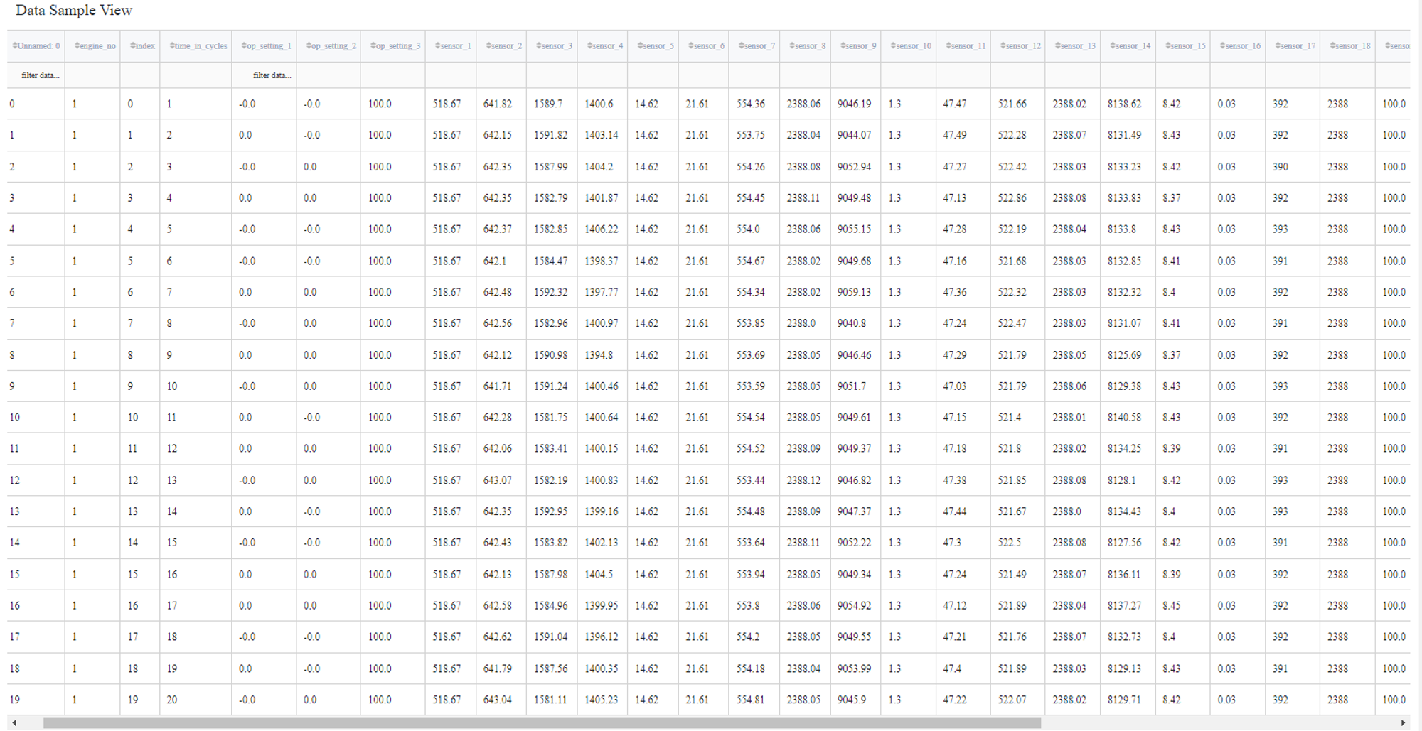
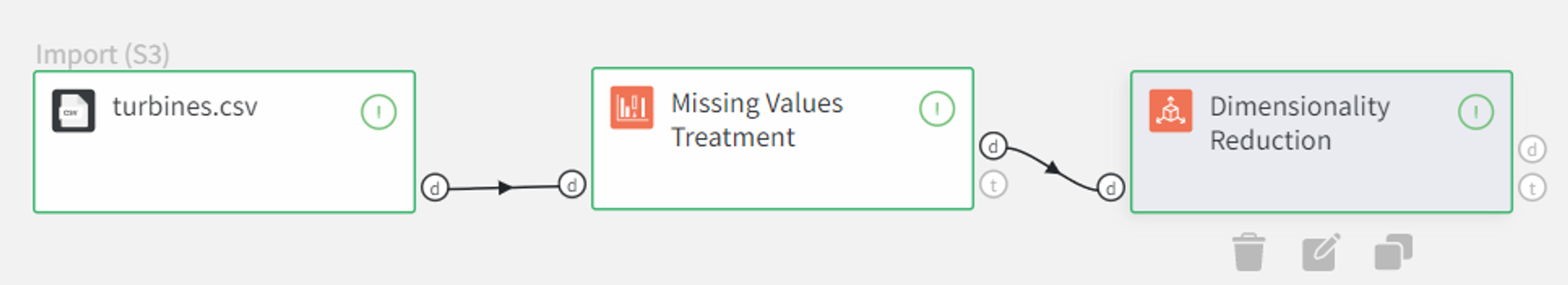
Let’s have a look at how it works on the ‘turbines.csv’ dataset.

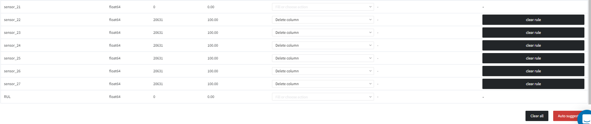
First, we need to handle the missing values using the ‘Missing Values Treatment’ Brick. Columns that are filled with nan values are deleted.
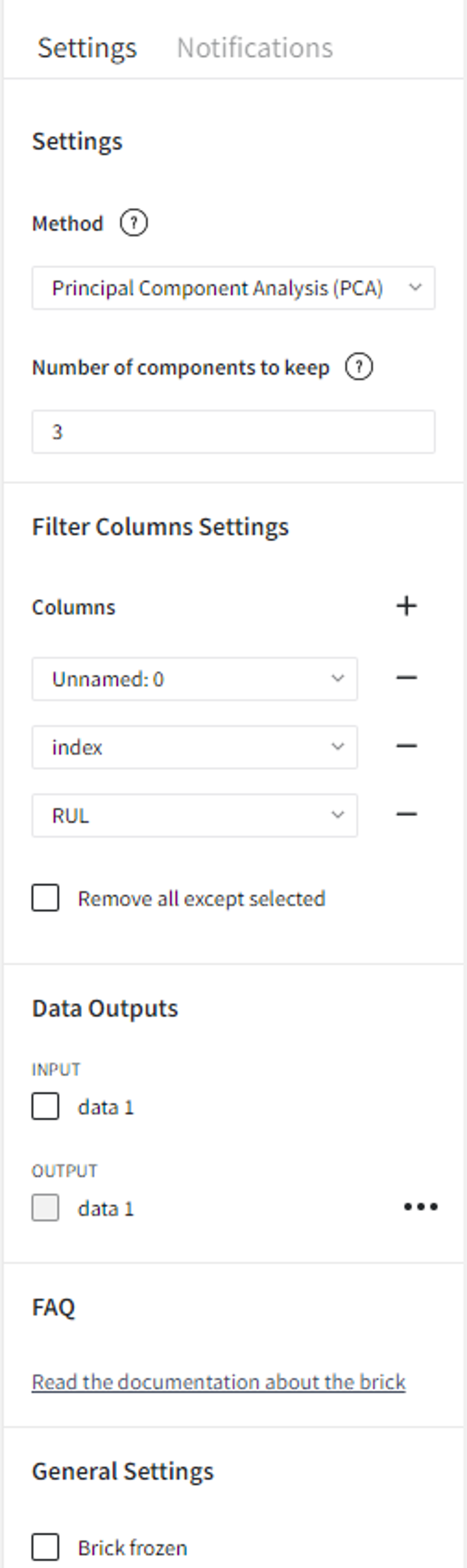
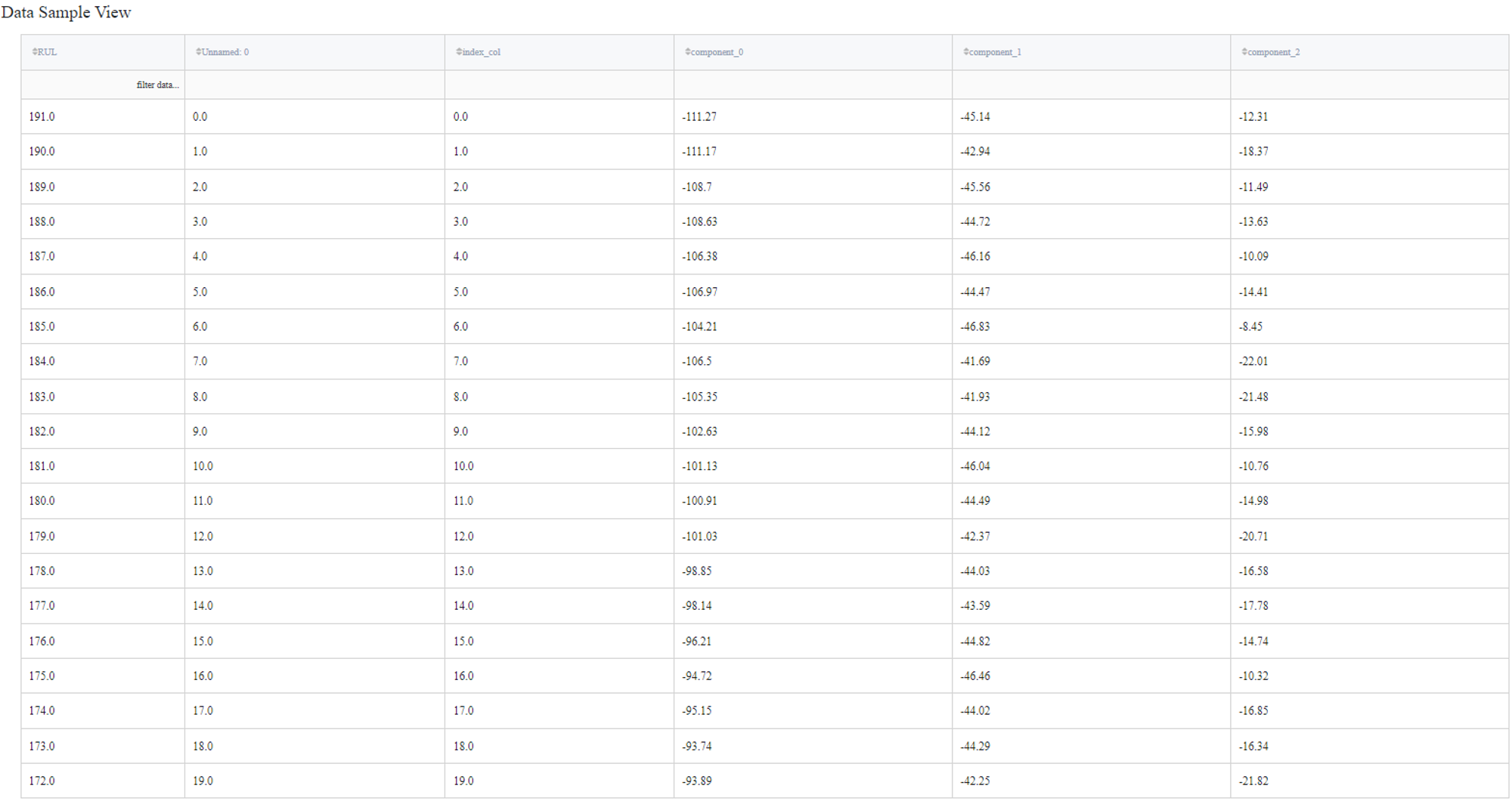
Now we can apply the ‘Dimensionality Reduction’ brick with PCA method, 3 dimensions to keep and filter columns ‘Unnamed: 0’, ‘index’, and ‘RUL’.
After setting the configuration we can run the pipeline and see the results in the Output section on the right sidebar. We got a new dataset with the columns we kept with no change and 3 new columns ‘component_0’, ‘component_1’, and ‘component_2’ that represent the input features.
After a successful pipeline run, the transformer asset can be saved by clicking the ‘Save’ button and reused later.