General information
DBSCAN (Density-based spatial clustering of applications with noise) is a popular unsupervised machine learning algorithm, which groups together points that are close to each other. It also marks points that are in low-density regions as outliers.
Its benefit is that it doesn’t require to specify the number of clusters and it can find arbitrarily shaped clusters.
DBSCAN algorithm classifies every data point into 3 categories: core point, border point, and outlier. It generally takes two parameters: ‘epsilon’ (the maximum distance between two samples for one to be considered as in the neighborhood of the other) and ‘minPoints’ (the number of samples in a neighborhood for a point to be considered as a core point including the point itself). For every data point, if it has at least ‘minPoints’ within ‘epsilon’ distance, it is a core point. If there are fewer than ‘minPoints’ within ‘epsilon’ distance but the point is in the neighborhood of a core point, then it’s a border point. In other case, the data point is an outlier. For locating data points in space, DBSCAN mostly uses Euclidean distance, although other methods can also be used.
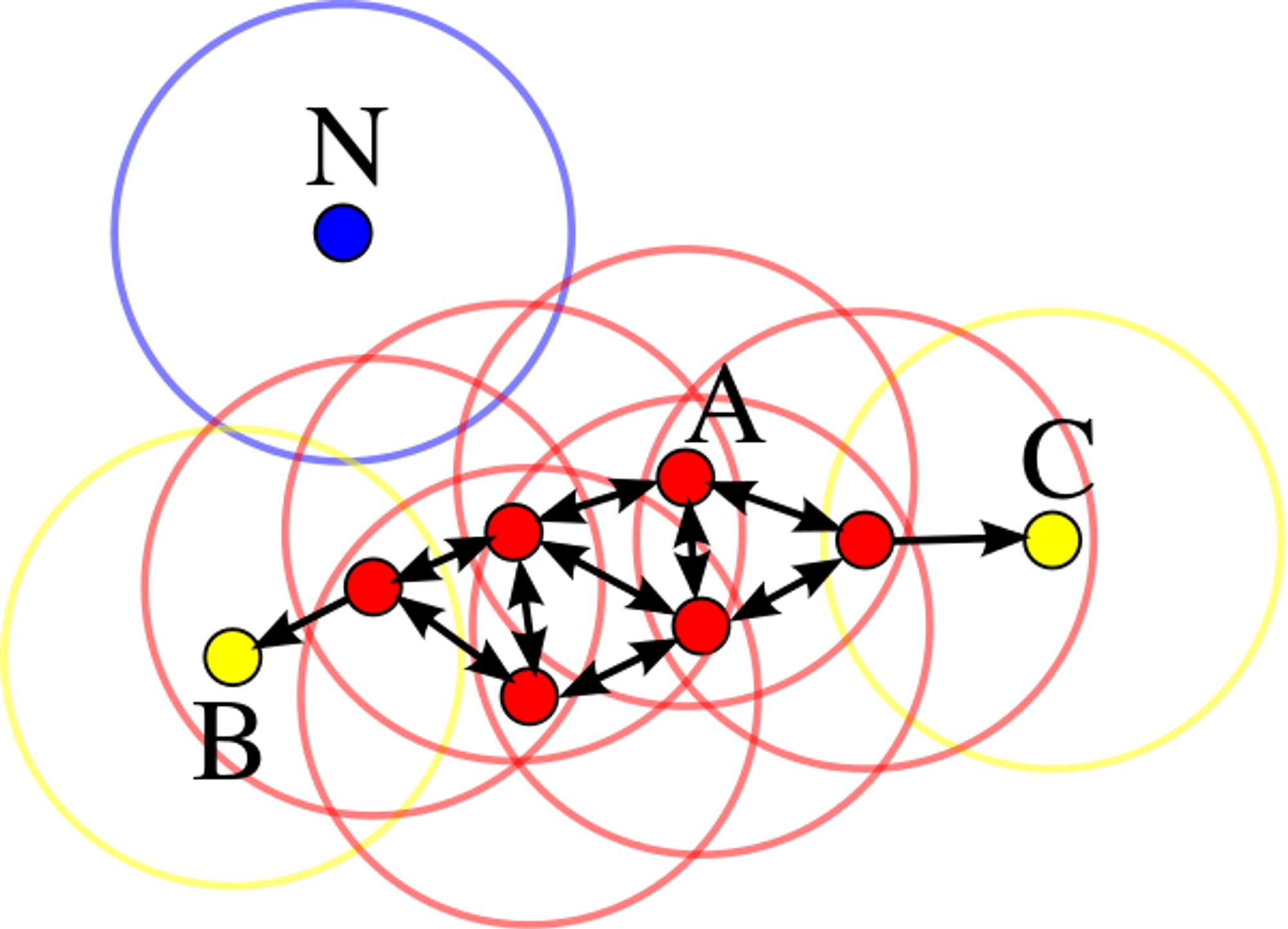
Example for minPoints=4
A cluster includes core points that are neighbors (i.e. reachable from one another) and all the border points of these core points.
Description
Brick Locations
Bricks → Machine Learning → DBSCAN Clustering
Brick Parameters
- Epsilon
The maximum distance between two samples for them to be considered as neighbors.
- Columns
Columns that are removed from the dataset for clustering. However, they will be present in the resulting set. Multiple columns can be selected by clicking the + button.
In case you want to remove a large number of columns, you can select the columns to keep and use the flag ‘Remove all except selected’.
Brick Inputs/Outputs
- Inputs
Brick takes the dataset
- Outputs
Brick produces the dataset with an extra column called ‘predicted_cluster’, where cluster ‘-1’ indicates the outlier and other cluster labels have integer values starting from ‘0’.
Example of usage
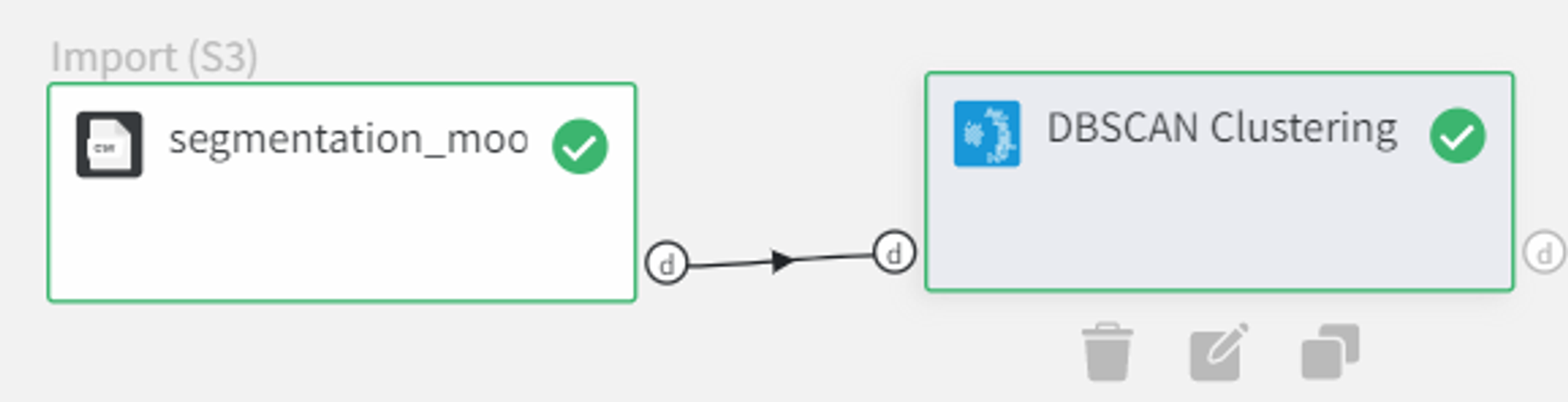
Let’s try to segment data from the ‘segmentation_moons.csv’ dataset using DBSCAN algorithm. The dataset consists of 3 columns: ‘Unnamed: 0’, ‘0’ and ‘1’.
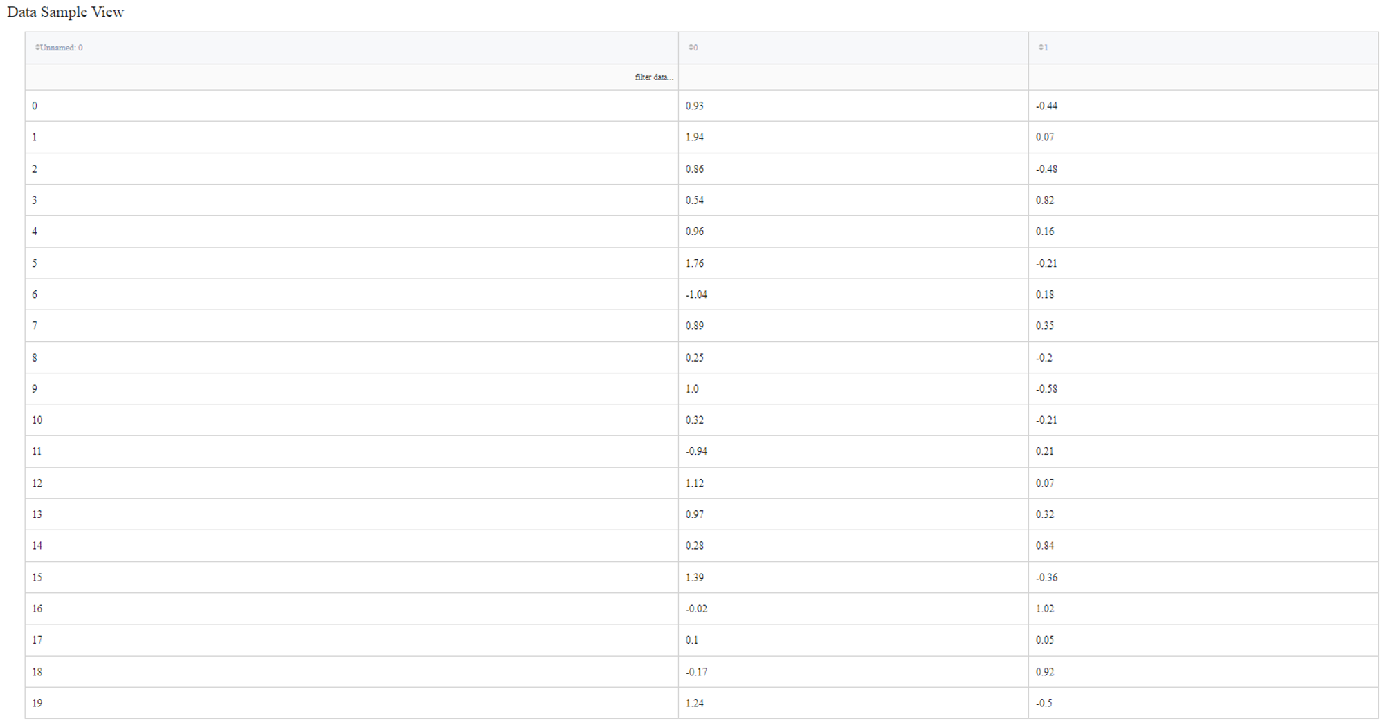
So we connect this dataset directly to the DBSCAN Clustering Brick, set ‘Epsilon’ equal to 0.1, filter column ‘Unnamed: 0’ as it sets the index of the record and doesn’t represent any feature of the sample. After configuring the settings we can run the pipeline and see the results in the Output section on the right sidebar. We got the same dataset with an additional column ‘predicted_cluster’, which has values from -1 to 1. It means that we segmented our data into 2 clusters and points that were predicted as cluster ‘-1’ are the outliers.
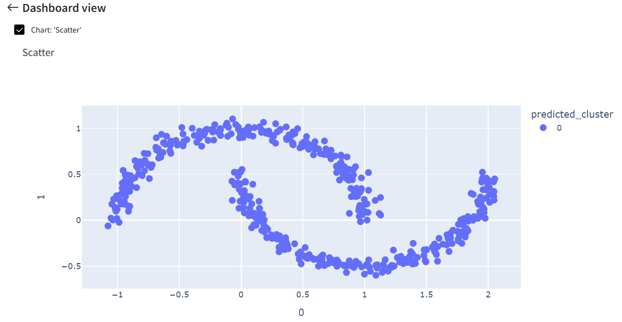
Let’s visualize the predicted clusters to see how the segmentation worked.
We can connect the output from the DBSCAN Clustering Brick into the Charts Brick and create a scatterplot with column ‘0’ on the X-axis, column ‘1’ on the Y-axis, and Color column → ‘predicted_cluster’ and run the pipeline again.
Finally, we can click ‘Open dashboard view’ and see the following segmentation visualization:
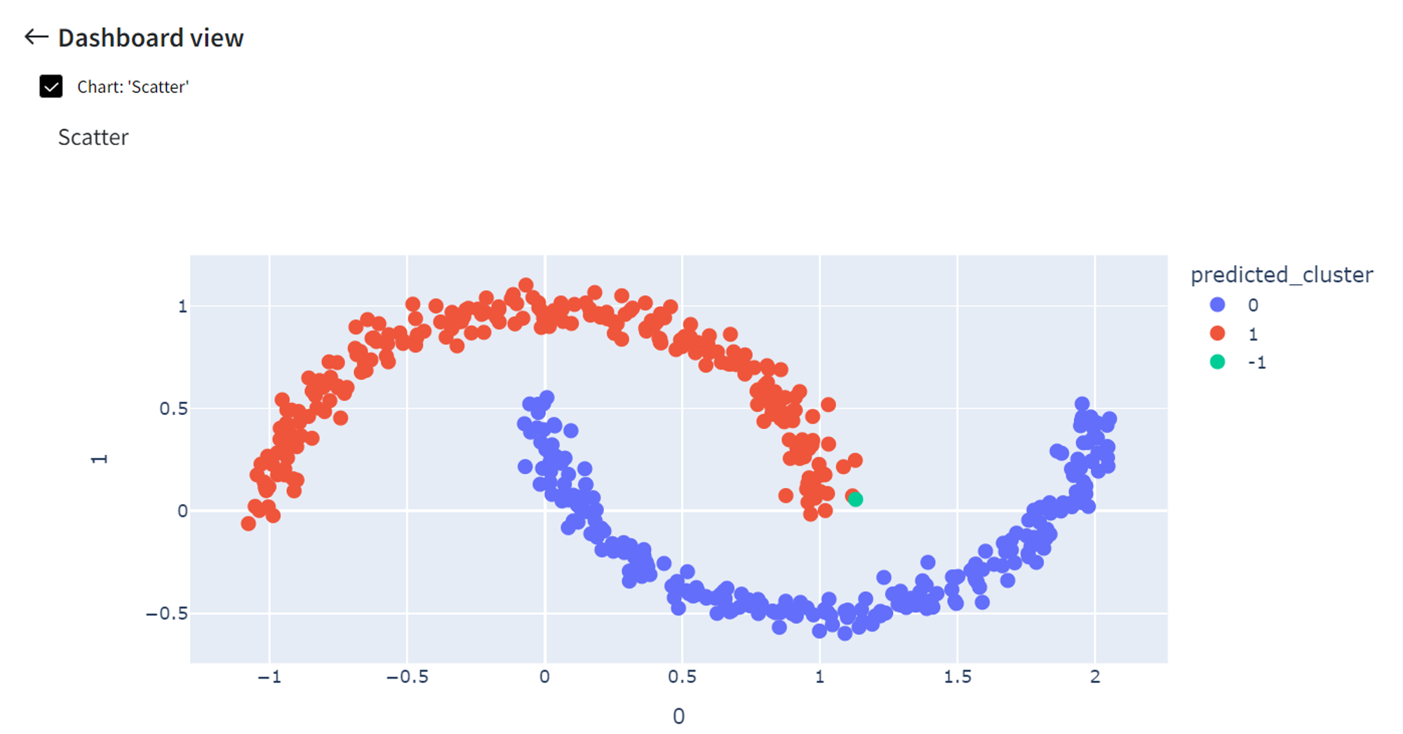
It did pretty well segmenting the moon-shaped clusters while in this case, for example, K-means clustering would give much worse results.
If we try to experiment with ‘Epsilon’ values we will get some intresting results.
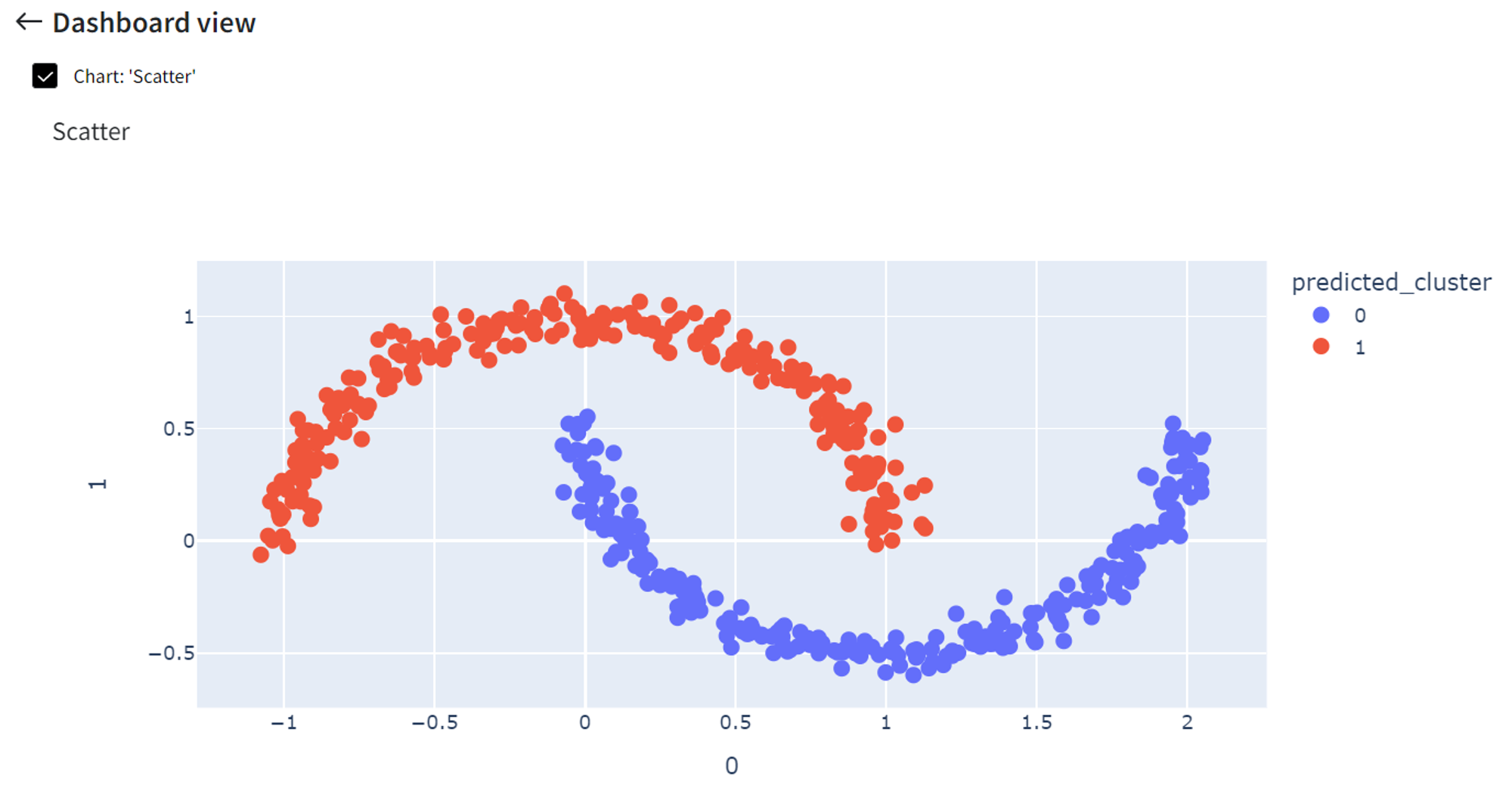
For example, if ‘Epsilon’ = 0.2, we no longer have outliers in our dataset, but the number of clusters and their appearance stays the same.
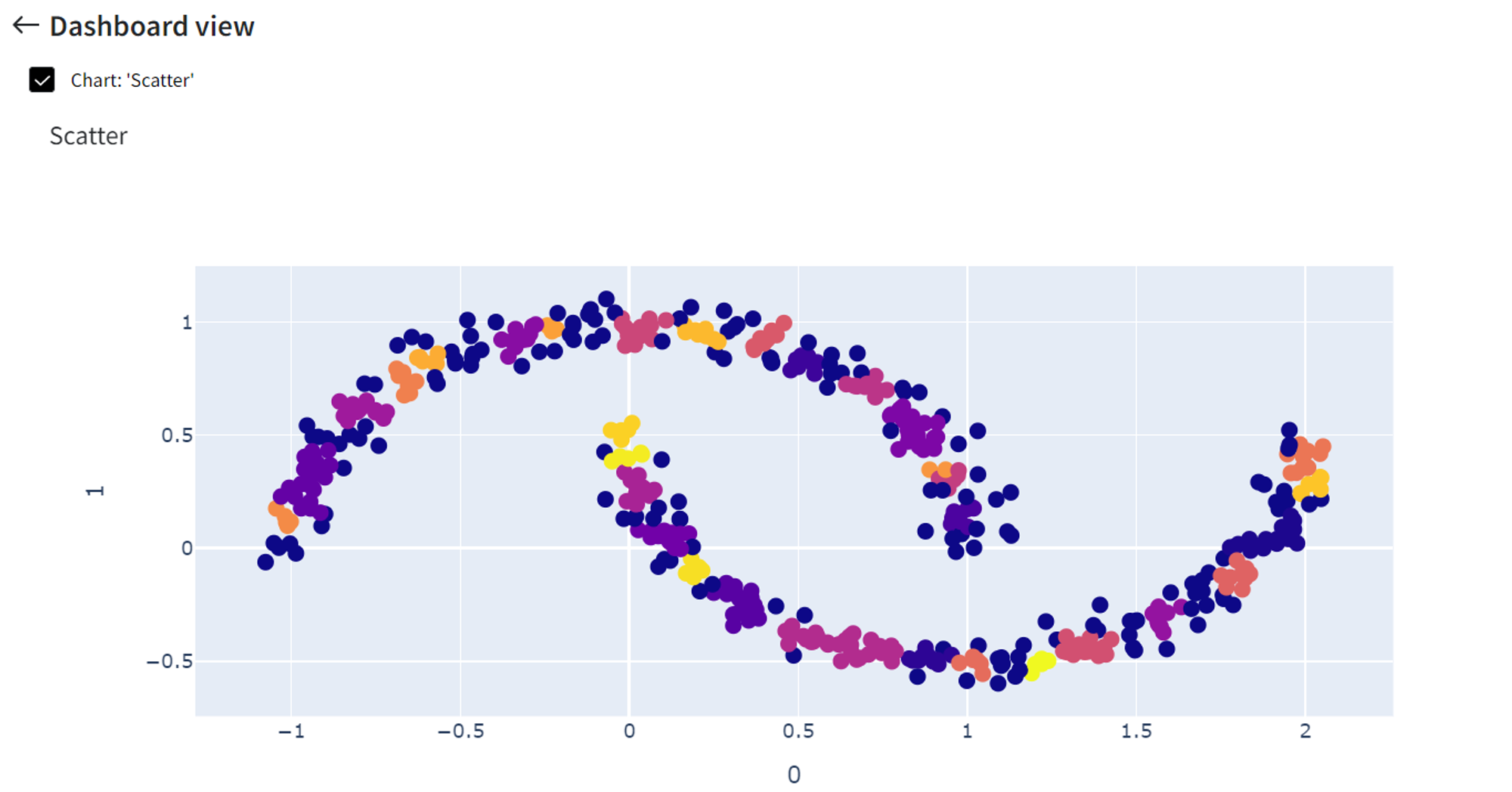
If ‘Epsilon’ is a small number, like 0.05, only very close points are grouped, so we get around 32 different clusters.
On the other hand, if ‘Epsilon’ is too large, for instance 0.4, then we include everything in a single cluster.