General Information
Time-series forecasting is one of the important machine learning applications strongly connected with various business domains - from Retail and Finance to Manufacturing and Predictive Maintenance. There are many cases when the predictive problem requires time components involvement, especially when the prediction is related to the processes that change over time. These dependencies can be identified and analytically described.
In time series forecasting, we are using the model to predict the future values of the target numerical variable based on its historical data - previously observed values. It is essential to differentiate the regression analysis and time series forecasting. While the regression is aimed to describe the relationships between two or more numerical variables (time series), the time series forecasting reconstructs the relationships between different points in time within the same series. There are some typical examples:
- Forecast stocks prices based on the analysis of the historical observations
- Forecast customers interest rate
- Weather forecasting
- Forecasting machinery failures in predictive maintenance
Data Processing pipeline
Time Series Forecasting brick provides the possibility to train and apply the forecasting model based on the analysis of historical time-series data with the inline capabilities of its preprocessing. Brick processing pipeline consists of three parts:
- Time Series feature extraction
- Trend and Seasonality
- Data logging time parameters
- Additional regressors
- Negative target values support
- Forecasting horizon detection
Time series data is represented by using the additive model:
where
- a non-linear trend that reflects long-term increasing or decreasing data.
- seasonality, some patterns, occurring when a time series is affected by seasonal factors connected with yearly, weekly, or daily activity so that the time-series can be characterized by corresponded seasonality.
-noise, which describes random, irregular influences that can't be explained by trend and seasonality effects.
Seasonal effects are defined automatically, but the manual settings are also supported.
Data gathering usually has some logging frequency, and we may extract this information to understand the optimal discretization step and the missing time-steps diagnostic.
Regressors are the extra features that provide additional information about factors that impact the forecasted variable and are known in the past and the future. As there is a possibility to use any numerical columns as regressors, the brick assesses their predictive abilities regarding the target variable and chooses the variables that meet the predictability requirements.
In many business applications, we do not operate with the negative values of the forecasted variable, like in the case of demand level, customer interest rate, currency exchange rate. It is a minimal list of the situations when the target variable can not take the negative values, so we may preliminary analyze the data and identify if there is a necessity to apply the non-negative prediction restrictions.
The optimal forecasting horizon depends on the time-series structure - the length of the historical data, seasonality, cycling components, and forecasting model's parameters - all of these factors are considered to apply the trained model to make the forecast.
- Preprocessing time-series before modeling
- Outliers Treatment
- The Discretisation of Time Series data that supports several aggregation methods
- Time Steps - minutes, fourth, days, month, year
- Method - min, max, mean, median, sum, first, last
- Filling the missing dates
- Treatment of the missing values in the target variable
If the time series has the point-type outliers they can be detected by using the median average approach:
The abnormal cases are changed to the estimated median value.
The processed time series can be converted to specific time-step observations like hours or days and depicts the general behavior for the observed period. For instance - the average daily temperature, or the total sum of the sales product items per week. Time Series forecasting brick supports the following aggregation configuration:
Time series might have some gaps in the data logging that may be explained by the different reasons - from technical issues to the activity absence. In some cases, these gaps might be ignored, and the time series is passed to the model training as is, but there are cases when we are interested in leading the time series to the normalized view.
If the target variable has missing values, we should handle them via one of the proposed strategies: forward/ backward fill, linear interpolation, mean, and zero filaments. The first three strategies suppose the sequential processing of the time series, while "mean" and "median" allows to change all the missing values by one of the position statistics.
- Forecasting model fitting and applying
As a core of Time Series forecasting, we use the FB Prophet model (see Prophet brick). Model is trained on the prepared data and applied to the future with the saving the data structure.
The one more available functional configuration is Stratification. Stratification allows to set up of the column for the dataset stratification. This setting is optional and should be used in the case when the data contain several time-series, which describe the independent processes:
Example: The pharmacy chain management would like to improve their planning processes via demand forecasting in the different outlets. It means that we should gather the data that reflect the sales history for each pharmacy branch and analyze them independently.
Brick Usage
Time Series Forecasting supports two modes of usage:
- Simple mode - the user defines the target variable that should be predicted, the date-time variable that is the mandatory input variable and used as a time marker, and the variable for stratification (optional). In simple mode, the data preprocessing and the model hyper-parameters settings are performed automatically based on the dependencies extracted from the time series:
- Seasonality detection (daily, weekly or yearly)
- Aggregation based on the data logging time step
- Regressors auto-detection
- Outliers removing
- Treatment of the missing values of target variable and regressors
Simple Mode Configuration
Name
Enaibled
Method
- Advanced mode - the user gets the possibility to configure the brick with all advantages of the simplified mode, but without its limitations - we provide a very flexible combination of the manual and automatic configurations that allows introducing the expert knowledge to the time series processing pipeline
Advanced Mode Configuration
Name
Enaibled
Method
Description
Brick Location
Bricks → Machine Learning → Data Mining / ML → AutoML → Time Series Forecasting
Bricks → Machine Learning → Data Mining / ML → Time Series Forecasting → Time Series Forecasting
Brick Parameters
- Target Variable
The column that we want the model to predict. This variable should be numerical and depends on the DateTime variable.
- Date Column
The column contains the independent DateTime variable, which is the basis of the Time Series data.
- Stratified by
A column with the Stratification key is used to divide the dataset into independent time series and train the models for each stratum independently (see For-Loop).
- Disallow negative predictions
Advanced option. This checkbox forces the model to round up negative predicted values to be set to 0.
- Seasonality
Advanced section. Manual settings of the seasonal effects should be handled by the model (yearly, weekly, and daily). Seasonality settings may include all of these periods as well as don't contain any of them.
- Regressors Settings
Advances section. This section is aimed at the additional regressors list composition.
Auto-detection
The checkbox allows switching between manual and auto regressors detection. When auto-detection is off, the potential regressors are selected manually and cannot be defined at all.
Columns
List of possible columns for selection. It is possible to choose several columns for filtering by clicking on the '+' button in the brick settings.
- Missing target treatment
- forward fill (default) - the missing values are filled by the latest valid observation
- backward fill - the missing values are filled by the subsequent valid observation
- linear interpolation - the missing values are restored by values that reflect the linear trend between the nearest valid observations.
- mean - the missing values are filled by the calculated average of the target variable
- zero- the missing values are filled by zero value
Advanced section. The section for configuring the method for the treatment missing values in the target variable.
Fill missing target
Missing target treatment method configuration. The user can select one of the following:
- Remove outliers
Advanced option. The binary flag allows enabling/disabling of the time series outliers detection and removing
- Aggregation
- auto (default) - aggregation is based on the initial logging time steps
- minutes - the time steps will be set to the minute granularity and used as the aggregation key
- hours - the time steps will be set to the hour granularity and used as the aggregation key
- days - the date-time will be transformed to date format (without time markers)
- month - the time series will represent monthly dynamic
- year - the time series will represent yearly dynamic
Advanced section. Section for applying the custom strategy to the time series discretization.
Enable aggregation
The binary flag allows enabling/disabling the time series discretization.
Step
Aggregation key. The time step defines the distance between the nearest points in the aggregated dataset. There are the following options:
Method
Statistics that represents the time series after discretization (min, max, mean, median, sum, first, last)
- Missing dates treatment
- frequency-based - the restored dates are defined via logging frequency assessment
- time-based - the restored dates are based on the logging time granularity
Advanced section. The section for configuring the approach to remove the time gaps.
Fill missing dates
The binary flag allows enabling/disabling the missing dated treatment step.
Method
Missing dates treatment method configuration. The user can select one of the following:
Brick Inputs/Outputs
- Inputs
Brick takes the data set that has the time series structure.
- Outputs
- Data - modified input data set with added columns for predicted classes or classes' probability. Dataset structure may differ from the initial dataset because of the preprocessing stage.
- Model - a trained model that can be used in other bricks as an input
Brick produces two outputs as a result:
Outcomes
- Forecasting Dashboard
- Supported metrics: RMSE, MAPE, R2
- Supported charts: Prediction/Distribution plot, Q-Q plot, Prediction Error Analysis plot, Residual plot
Integration of the Forecasting Dashboard to the Model Output dashboard. The dashboard allows seeing the results of the target variable forecasting without the necessity to use the separate dashboard.
Model Performance
The dashboard provides detailed information about the quality of the forecasting model.
- Time Series Processing
- stratification - the name of the stratification column (None if was not defined)
- summary - he detailed information about the data processing stages. If the stratification was used, this section would contain the information about each stratum
- aggregation - time series discretization summary
- aggregate - the binary flag that depicts that the aggregation performed.
- step - aggregation step (see Step documentation)
- statistics - aggregation function that was used for the columns representation in the discretized time series. The type of the function depends on the variable role in the time series:
- non-target categorical - first
- non-target numerical - mean
- target variable - according to the configuration
- outliers_treatment - time-series outliers treatment summary
- remove_outliers - the binary flag (true if outliers treated)
- number_of_outliers - the number of the detected outliers
- outliers - time steps list that is related to the outliers
- missing_dates_treatment - time-series gaps removing summary
- fill_missing_dates - the binary flag that indicates if the missing dates filled
- method - the missing dates treatment strategy
- missing_values_treatment - missing values treatment strategy that applied to the regressors ant target variable
- model_regressors - the list of the additional regressors
- exclude_stratum - the list of the strata excluded from the analysis due to the lack of the observations in the corresponded time series.
Time Series processing section contains the detailed information about data preprocessing before the modeling that is defined by brick configuration:
- Save model asset
This option provides a mechanism to save your trained models to use them in other projects. For this, you will need to specify the model's name, or you can create a new version of an already existing model (you will need to specify the new version's name).
- Download model asset
Use this feature to download the model's asset to use it outside the Datrics platform.
Example of usage
Let's consider the classical Time Series problem like Demand Forecasting. For this purpose, we take the "Rossmann Store Sales" dataset and train the model, which predicts the number of the sold items for each store with respect to the calendar parameters.
Executing simple-mode pipeline
The time Series forecasting brick supports the simple mode execution, so we may take a dataset with time-series data and pass them to the Time Series Forecasting brick without preliminary analysis and preprocessing:
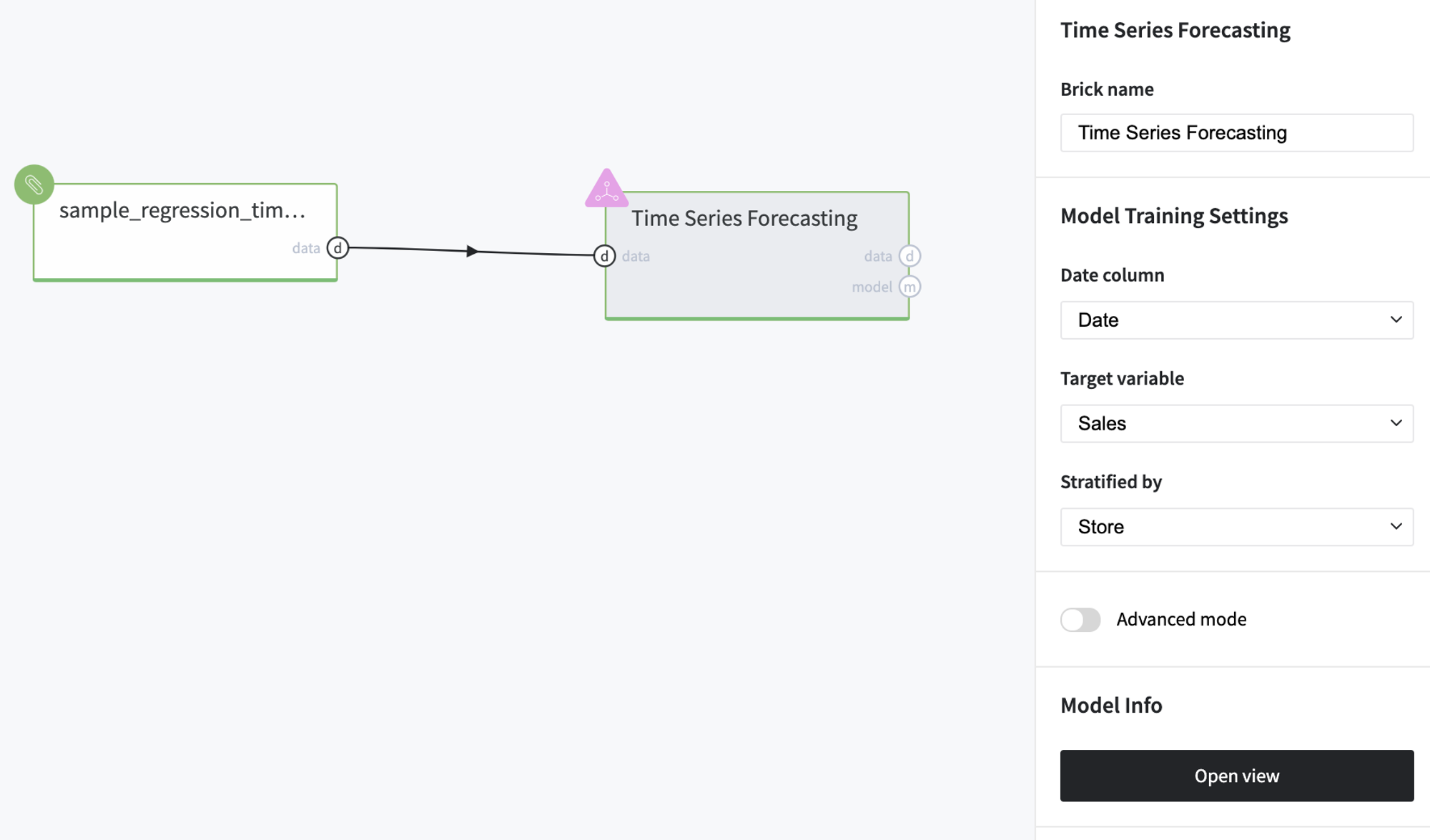
- First, drag-n-drop sample_regression_time_series_rossmann.csv file from Storage→Samples folder and Time Series Forecasting brick from Bricks → Machine Learning → Data Mining / ML → Time Series Forecasting → Time Series Forecasting.
- Connect the data set to Time Series Forecasting brick and define date-time, target, and stratification variables:
- Date column - Date
- Target variable- Sales
- Stratified by - Store
- Run pipeline and press Open View to see the model dashboard
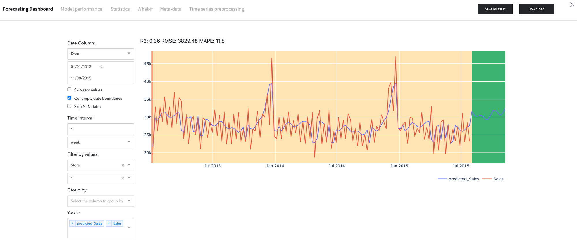
Model Results
- The result of the time series forecasting is showed in the Forecasting Dashboard:
We may see the expected (blue) and predicted (red) demand levels on the diagram. The green area corresponds to the forecasted number of sold items for the selected store.
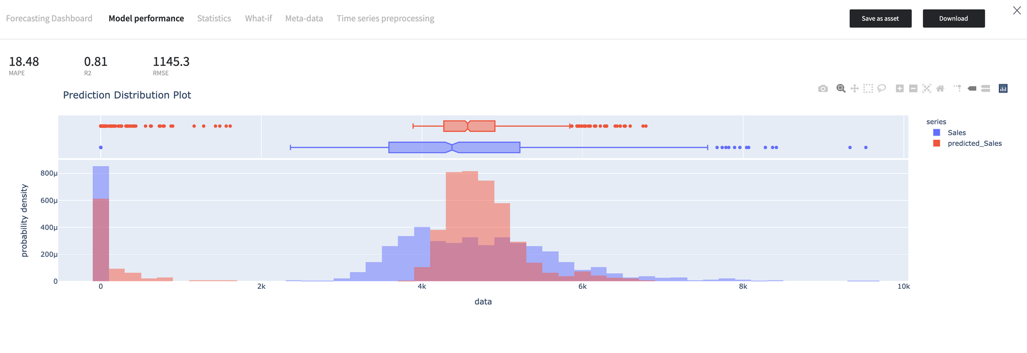
- The Model Performance dashboard represents the model quality assessment results.
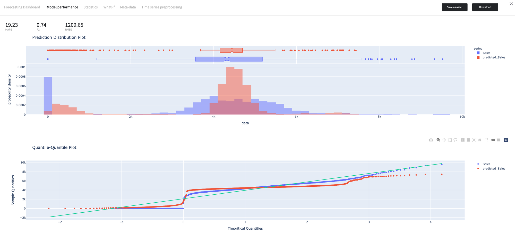
As we can see, the model predictions have a more peaked distribution, while the quantiles distribution is equivalent of the, which explains the R2 score is 0.74.
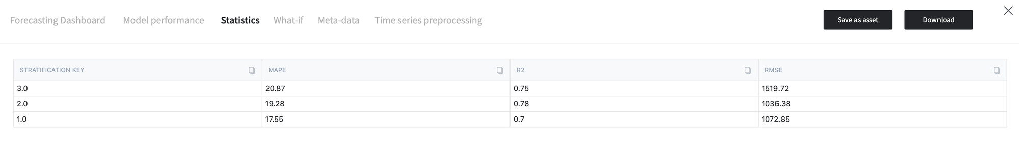
- The tab "Statistics" represents the quality of the model per each value of the stratified variable.
Finally, the Time Series Processing tab describes the data processing steps, as explained above.
Time Series Processing
{
  "stratification": "Store",
  "summary": {
    "3.0": {
      "aggregation": {
        "aggregate": true,
        "step": "days",
        "statistics": {
          "Open": "mean",
          "Sales": "mean",
          "Store": "first"
        }
      },
      "outliers_treatment": {
        "remove_outliers": true,
        "number_of_outliers": 48,
        "outliers": [
          "2013-01-07",
          "2013-02-04",
          "2013-02-18",
          "2013-03-04",
          "2013-03-18",
          "2013-03-25",
          "2013-05-01",
          "2013-05-31",
          "2013-06-03",
          "2013-06-17",
          "2013-07-15",
          "2013-07-29",
          "2013-08-12",
          "2013-09-09",
          "2013-10-07",
          "2013-12-02",
          "2013-12-16",
          "2013-12-23",
          "2013-12-30",
          "2014-01-06",
          "2014-01-20",
          "2014-02-03",
          "2014-02-17",
          "2014-03-03",
          "2014-03-31",
          "2014-04-14",
          "2014-05-01",
          "2014-06-02",
          "2014-06-16",
          "2014-06-30",
          "2014-09-01",
          "2014-09-15",
          "2014-09-29",
          "2014-10-06",
          "2014-11-03",
          "2014-12-01",
          "2014-12-15",
          "2014-12-22",
          "2015-01-05",
          "2015-02-02",
          "2015-02-16",
          "2015-03-02",
          "2015-03-30",
          "2015-05-01",
          "2015-05-18",
          "2015-06-01",
          "2015-06-15",
          "2015-06-29"
        ]
      },
      "missing_dates_treatment": {
        "fill_missing_dates": false
      },
      "missing_values_treatment": {
        "target": "ffill",
        "regressors": "ffill"
      },
      "model_regressors": [
        "Open"
      ]
    },
    "2.0": {
      "aggregation": {
        "aggregate": true,
        "step": "days",
        "statistics": {
          "Open": "mean",
          "Sales": "mean",
          "Store": "first"
        }
      },
      "outliers_treatment": {
        "remove_outliers": true,
        "number_of_outliers": 44,
        "outliers": [
          "2013-02-18",
          "2013-03-04",
          "2013-03-18",
          "2013-03-25",
          "2013-03-29",
          "2013-06-17",
          "2013-07-15",
          "2013-07-29",
          "2013-08-26",
          "2013-10-07",
          "2013-11-04",
          "2013-11-18",
          "2013-12-02",
          "2013-12-16",
          "2013-12-23",
          "2013-12-30",
          "2014-01-06",
          "2014-02-03",
          "2014-02-17",
          "2014-03-03",
          "2014-03-31",
          "2014-04-14",
          "2014-05-01",
          "2014-05-05",
          "2014-06-02",
          "2014-06-16",
          "2014-06-30",
          "2014-09-01",
          "2014-09-29",
          "2014-10-06",
          "2014-11-03",
          "2014-12-01",
          "2014-12-15",
          "2014-12-22",
          "2015-01-05",
          "2015-01-12",
          "2015-02-02",
          "2015-02-16",
          "2015-03-02",
          "2015-03-16",
          "2015-03-30",
          "2015-05-18",
          "2015-06-15",
          "2015-06-29"
        ]
      },
      "missing_dates_treatment": {
        "fill_missing_dates": false
      },
      "missing_values_treatment": {
        "target": "ffill",
        "regressors": "ffill"
      },
      "model_regressors": [
        "Open"
      ]
    },
    "1.0": {
      "aggregation": {
        "aggregate": true,
        "step": "days",
        "statistics": {
          "Open": "mean",
          "Sales": "mean",
          "Store": "first"
        }
      },
      "outliers_treatment": {
        "remove_outliers": true,
        "number_of_outliers": 37,
        "outliers": [
          "2013-01-07",
          "2013-02-04",
          "2013-02-17",
          "2013-03-04",
          "2013-03-18",
          "2013-03-25",
          "2013-03-29",
          "2013-05-02",
          "2013-05-13",
          "2013-05-31",
          "2013-07-15",
          "2013-07-29",
          "2013-12-01",
          "2013-12-15",
          "2013-12-22",
          "2013-12-27",
          "2013-12-30",
          "2014-01-06",
          "2014-01-20",
          "2014-03-03",
          "2014-04-14",
          "2014-04-18",
          "2014-05-02",
          "2014-06-02",
          "2014-06-20",
          "2014-11-02",
          "2014-11-24",
          "2014-11-30",
          "2014-12-07",
          "2014-12-14",
          "2014-12-21",
          "2014-12-27",
          "2015-01-05",
          "2015-03-30",
          "2015-04-03",
          "2015-05-01",
          "2015-07-27"
        ]
      },
      "missing_dates_treatment": {
        "fill_missing_dates": false
      },
      "missing_values_treatment": {
        "target": "ffill",
        "regressors": "ffill"
      },
      "model_regressors": [
        "Open"
      ]
    }
  },
  "regressors_list": [
    "Open"
  ],
  "excluded_strata": []
}
Interesting fact, that model the variable "Open" was selected as an additional regressor.
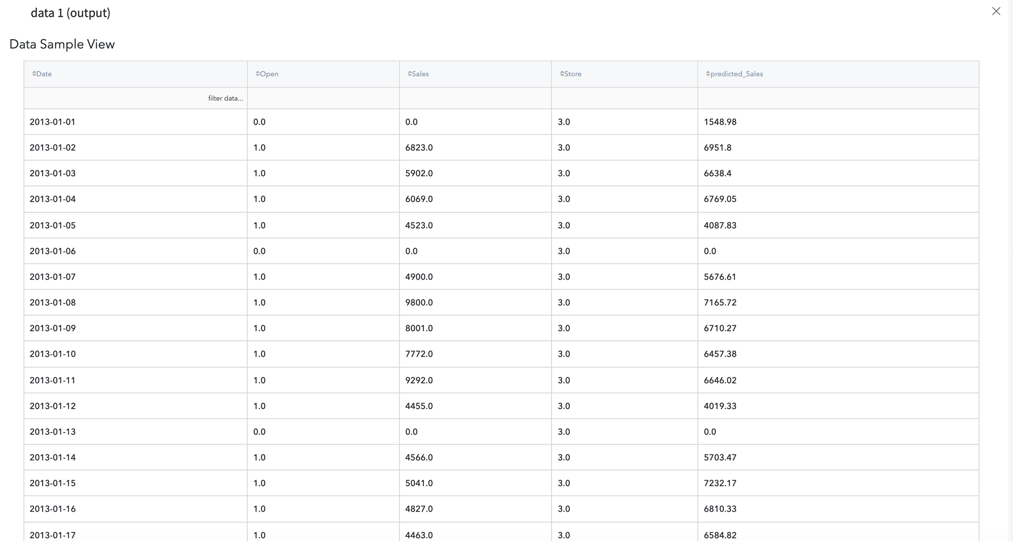
The obtained results are available for further analysis, and users have a possibility to review them via Output data previewer:
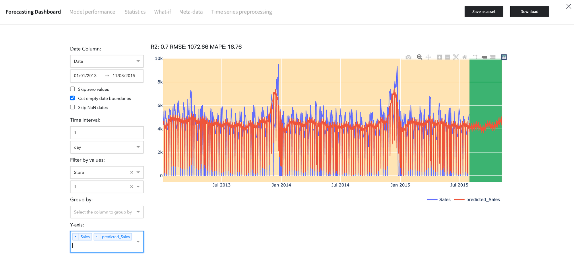
Executing advanced-mode pipeline
- Drag'n'drop sample_regression_time_series_rossmann.csv file from Storage→Samples folder and Time Series Forecasting brick from Bricks → Machine Learning → Data Mining / ML → Time Series Forecasting → Time Series Forecasting
- Connect the data set to Time Series Forecasting brick and define date-time, target, and stratification variables:
- Date column - Date
- Target variable- Sales
- Stratified by - Store
- Switch to the Advanced Mode
- Configure the brick:
Disallow negative predictions - True
Remove Outliers - False
Fill missing Target - Interpolation
Aggregation - days/sum
Results are depicted below: