Credit Scoring New

Description

Credit scoring represents an evaluation of the bank's customer creditworthiness - how well they can pay and are willing to pay off debt. According to the statistics, only less than one-half of the banked population regarded as eligible for lending, that's why they need for smarter credit scoring solutions is evident.

AI credit scoring decisions are based on a lot of data, such as total income, credit history, transaction analysis, work experience, etc. In essence, scoring represents a mathematical model based on statistical methods and accounting for a large amount of information. As a result, credit scoring using AI provides more sensitive, individualized credit score assessments based on an array of additional real-time factors, giving access to finance to more people with income potential.

Here we demonstrate the credit scoring assessment in Datrics platform, based on the data from open sources.

Problem Statement Dataset Modeling Scenario Datrics Pipeline Pipeline Schema Pipeline Scenario Dataset Preparation Data Preprocessing Feature analysis Modeling Results visualization Model Save and Deployment

Problem Statement

Create the Machine Learning model for the evaluation of the Credit Default Risk and build the ScoreCard for the new Customers' creditworthy assessment.

Dataset

For a demonstration of the credit scoring pipeline, we will use the subset of the Loan Club public dataset, which contains 10000 records with bank's customer information such as demographic and financial data provided for the loan request, loan details, credit history, and the current payment status.

This dataset is split into two separate files: lending_data.csv and member_rating.csv, which features are described below:

Dataset features for lending_data.csv

Feature

Description

acc_now_delinq

acc_open_past_24mths

Number of trades opened in past 24 months.

accept_d

The date which the borrower accepted the offer

addr_city

The address city provided by the borrower during loan application.

addr_state

The address state provided by the borrower during loan application

annual_inc

The annual income provided by the borrower during registration.

MORE FEATURES

Dataset features for member_rating.csv

Feature

Description

member_id

A unique LC assigned Id for the borrower member.

fico_range_high

The upper boundary of range the borrower’s FICO belongs to.

fico_range_low

The lower boundary of range the borrower’s FICO belongs to.

grade

LC assigned loan grade

sub_grade

LC assigned loan subgrade

Modeling Scenario

General Schema of the Customer Credit Scoring can be depicted as a sequence:

Gather the data with the target variable (loan_status) and features that can be used for the Customer's factors extraction

Encode the target variable and extract classes to predict

Generate features that can be useful for the creditworthy assessment

Transform and select the features that can be considered informative with respect to the target variable

Train and assess the Credit Default Risk model

Transform Model to the Scorecard and derive insights from the prediction

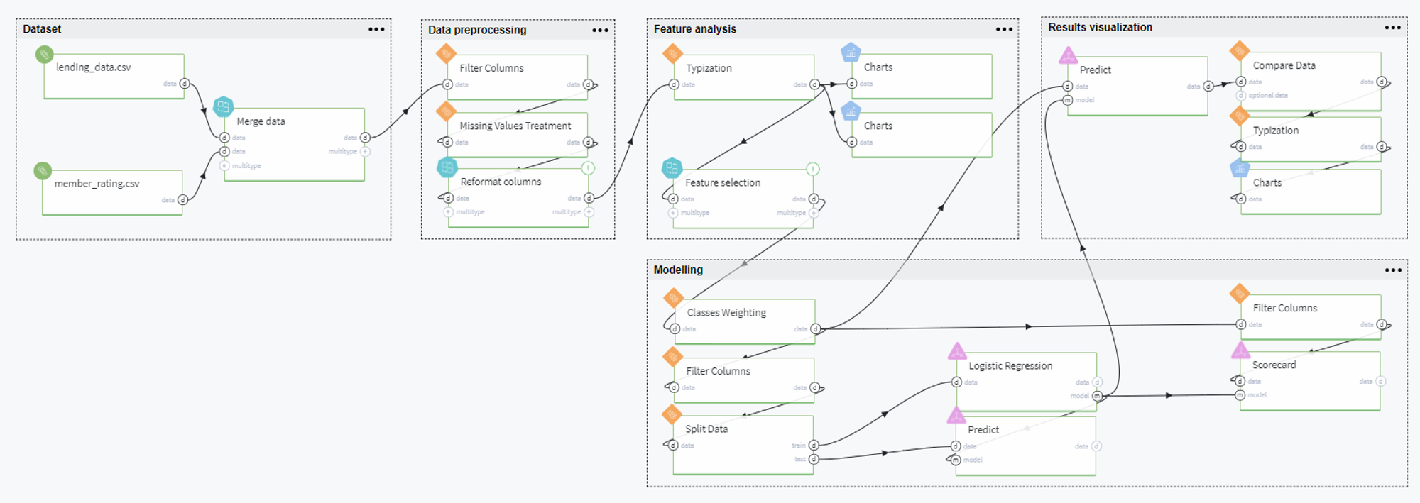
Datrics Pipeline

Pipeline Schema

The full pipeline is presented in the following way:

Pipeline Scenario

Overall, the pipeline can be comprised of the following steps: dataset preparation, data processing, feature analysis, modeling, and results visualization. Let us consider every step in detail below.

Dataset Preparation

BRICKS:

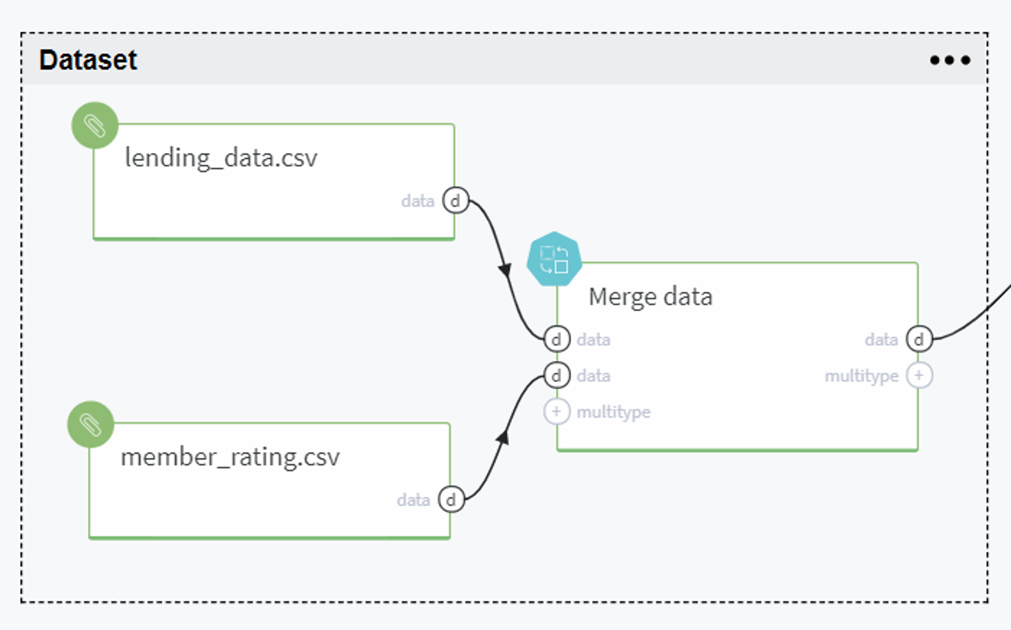
Pipeline

We start our model from loading the needed data and fitting it into the Pipeline brick that can be expanded in the following group of bricks:

BRICKS:

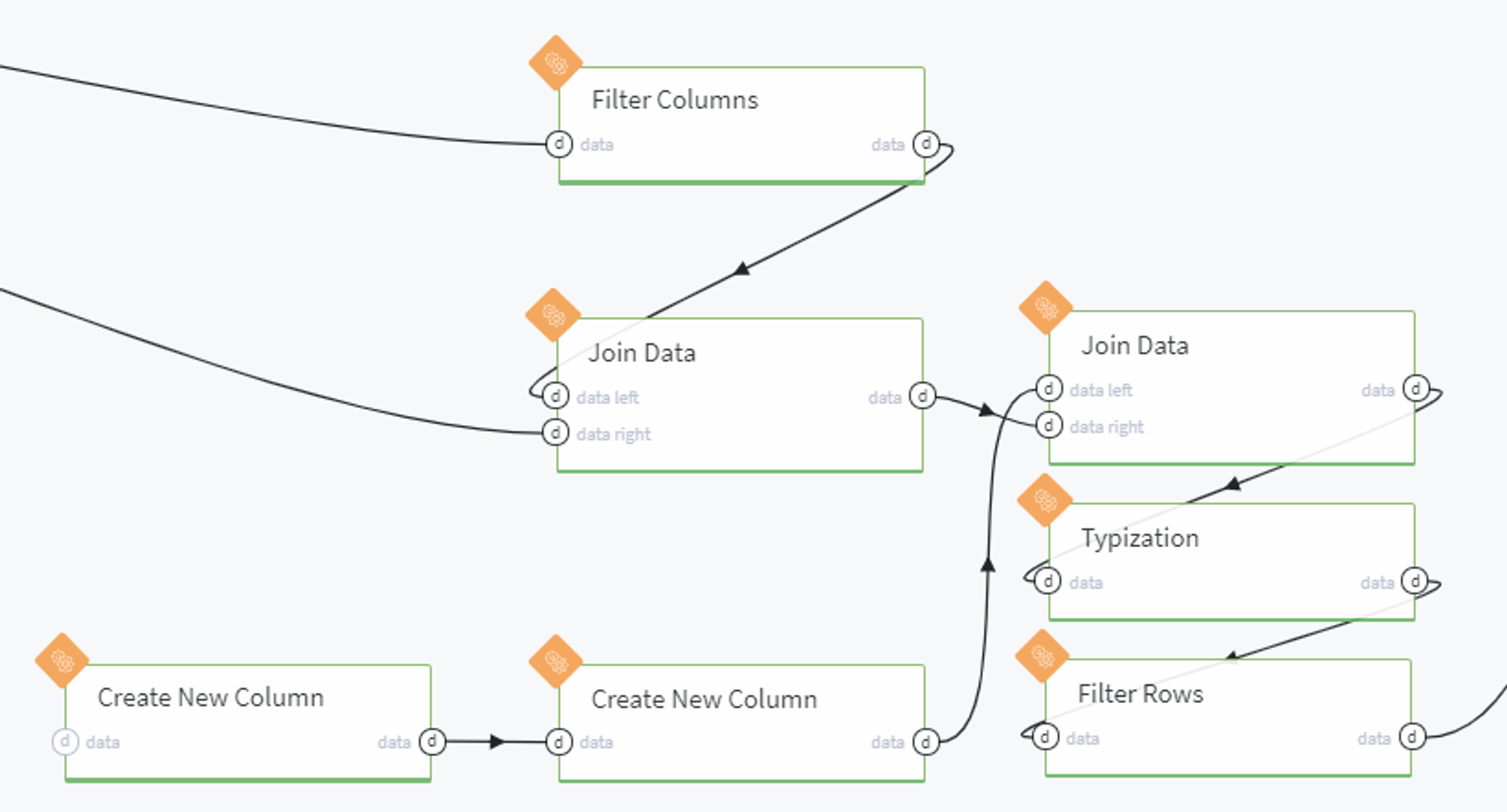
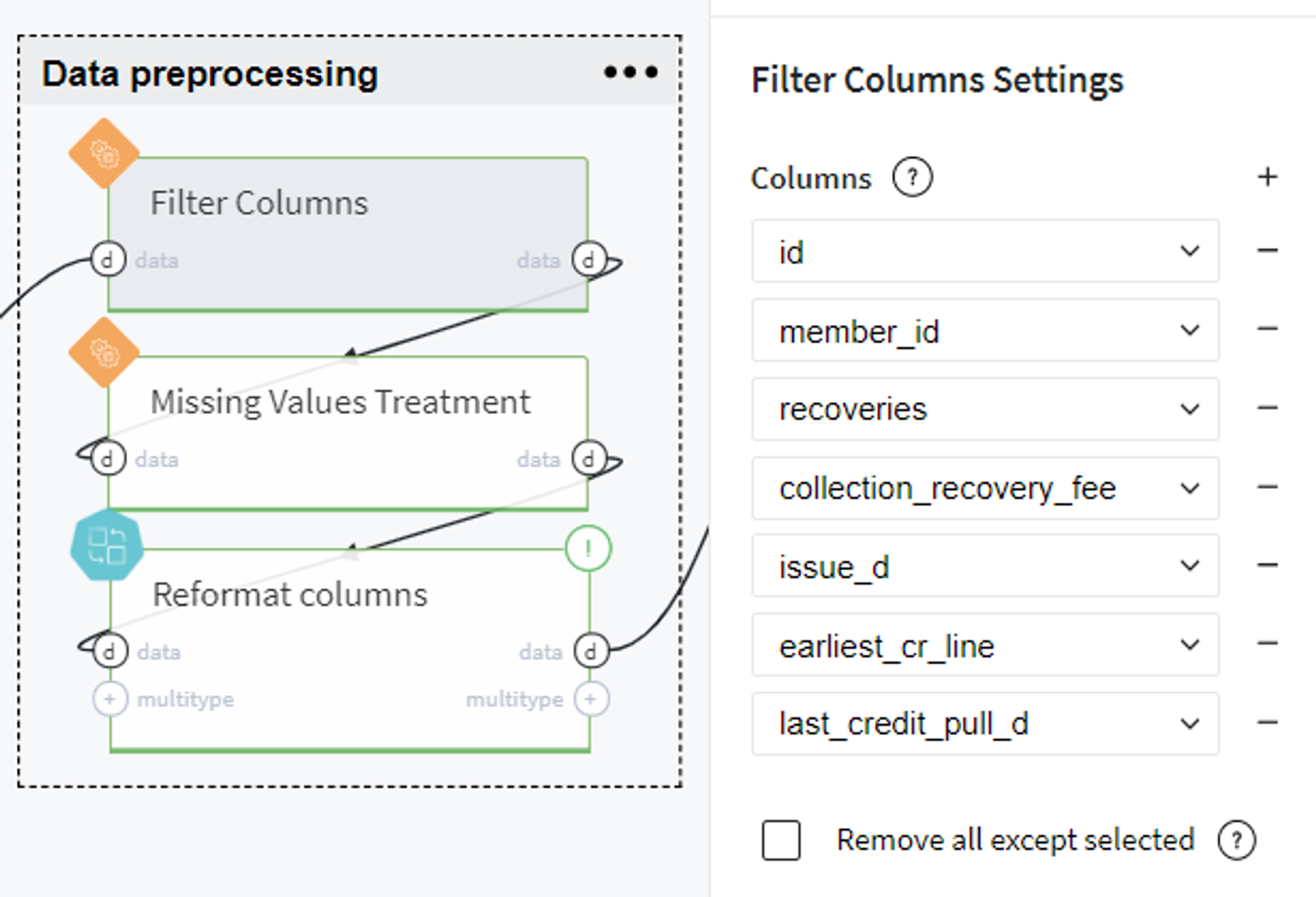
Here we, firstly, remove the forward-looking features which contain information about the current loan's payment statistics but are absent before the credit providing:

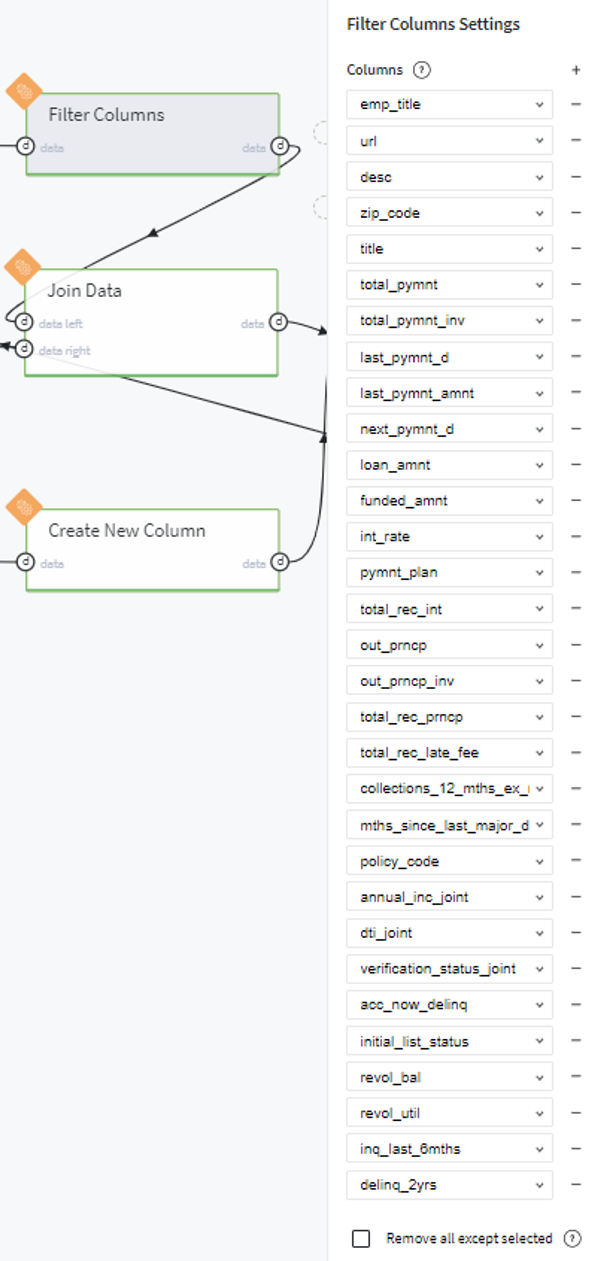
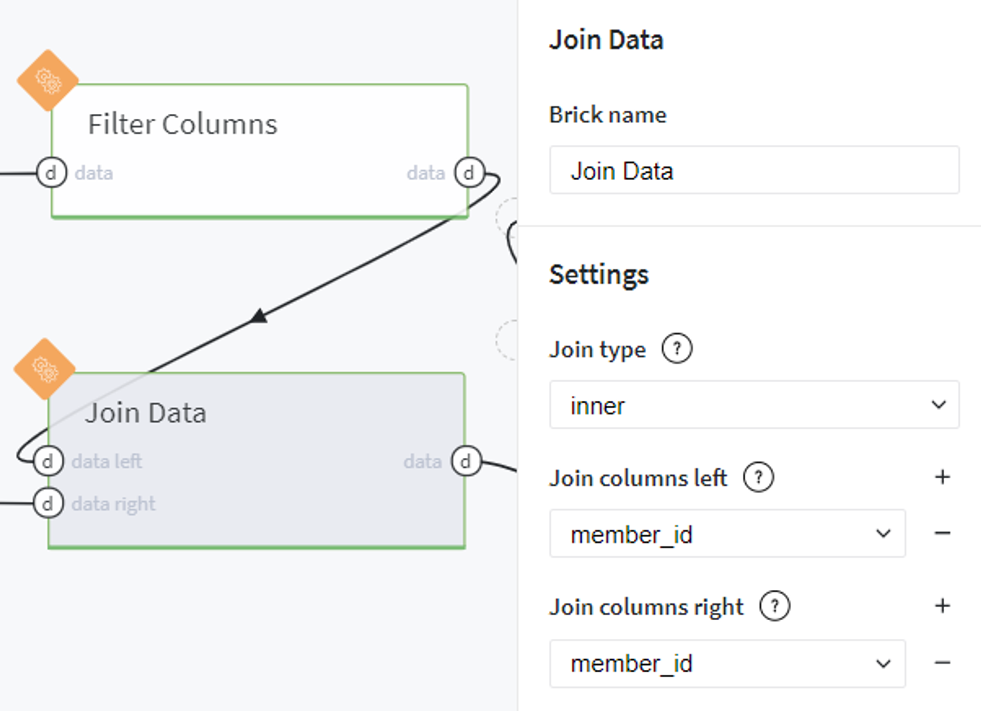
After that we join the filtered lending_data table with initial member_rating data by the member_id key:

At the same time we create a new dataset with all loan_status types available in the initial data (Charged Off, Default,Late (31-120 days), Does not meet the credit policy. Status:Charged Off, Current, Fully Paid, In Grace Period, Does not meet the credit policy. Status:Fully Paid, Late (16-30 days)):

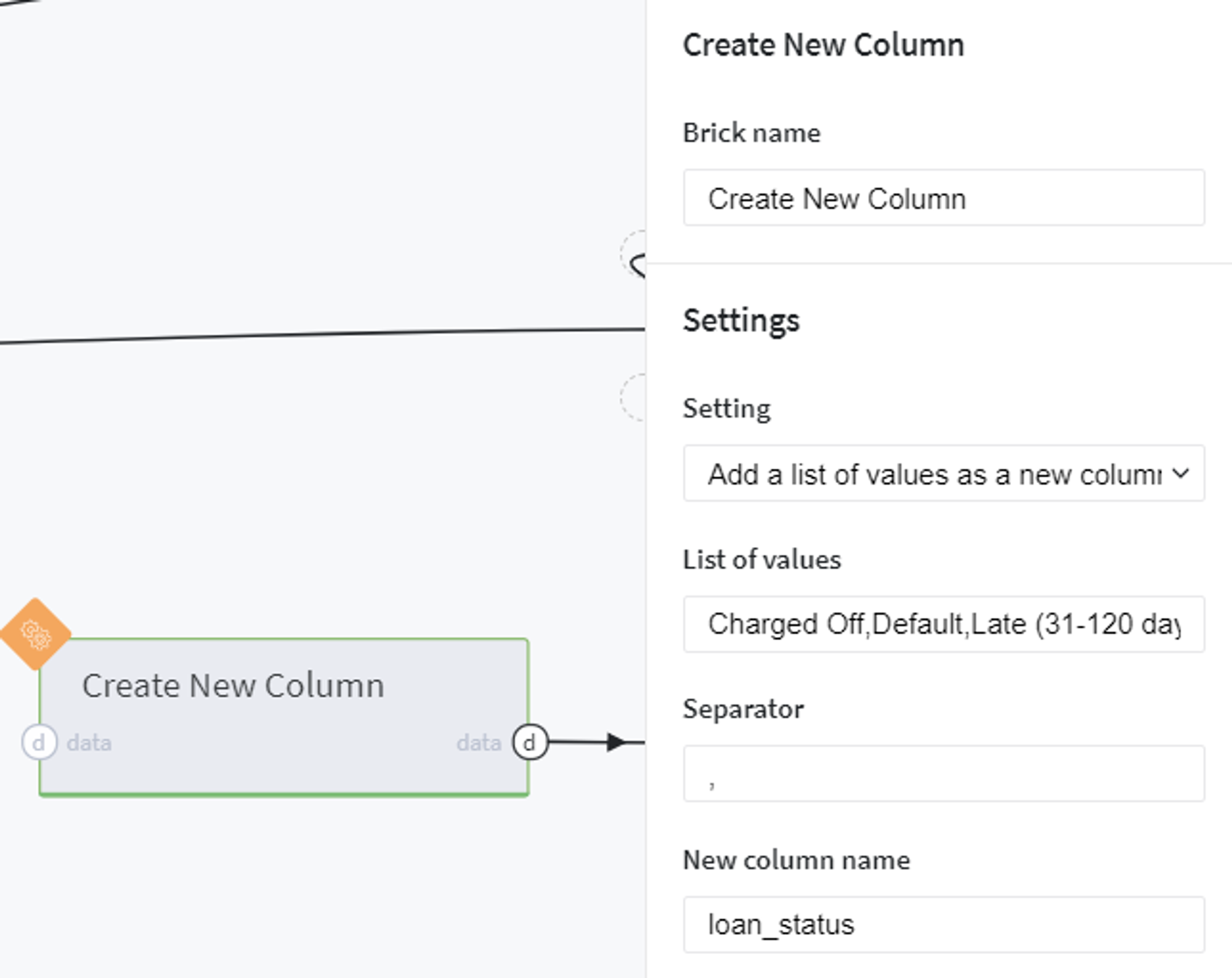
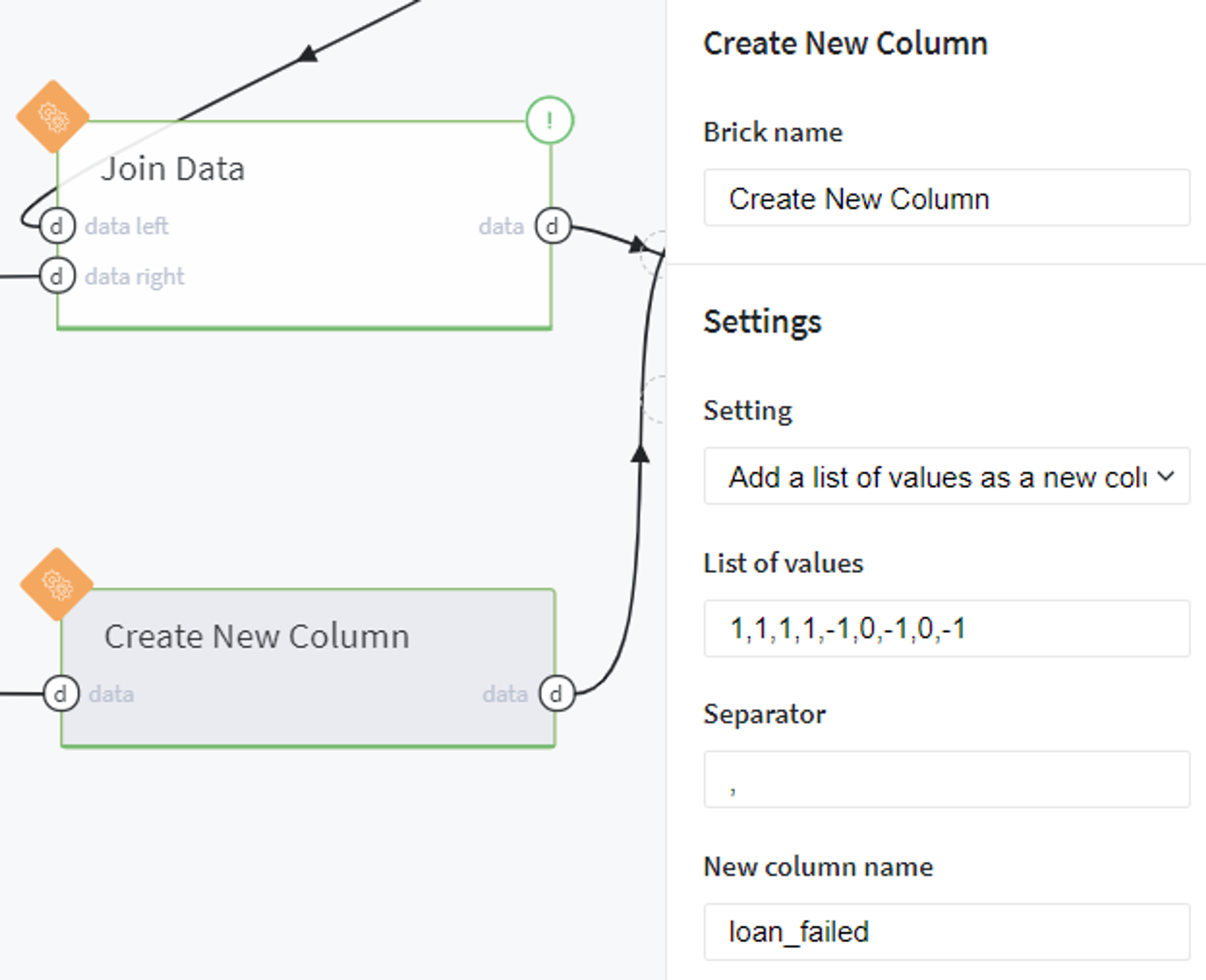
Then we define the binary target variable loan_failed as a new column of the created table with correspondence to the existing column loan_status:

The result must be as follows:

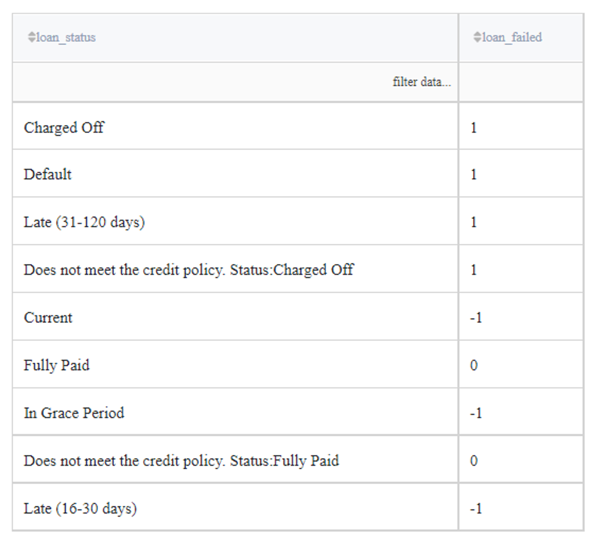
Note, that users that have the status Current, Late (13-30 days), or In Grace Period are considered as open cases (cases with uncertain results) and will be excluded from the analysis.

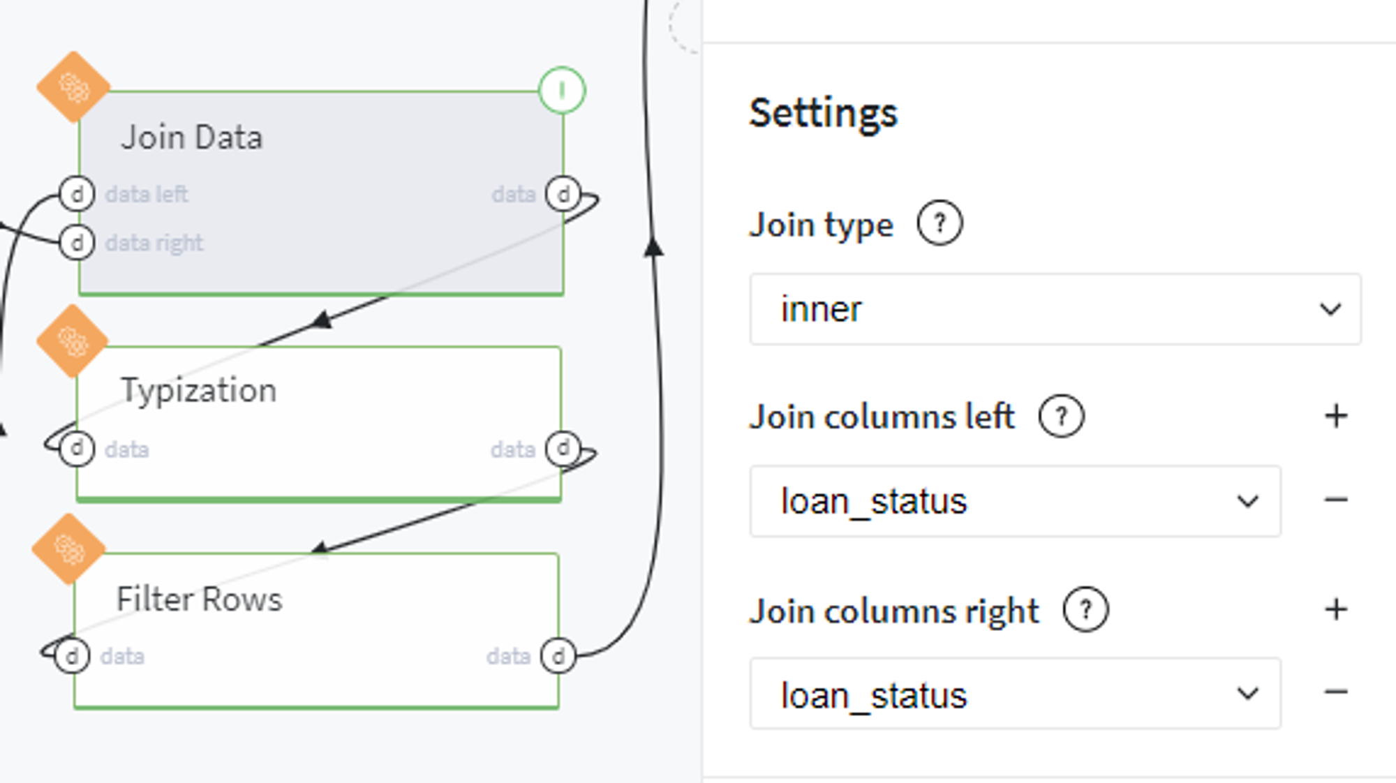
On the next step we join the newly created data with the full dataset by the loan_status key:

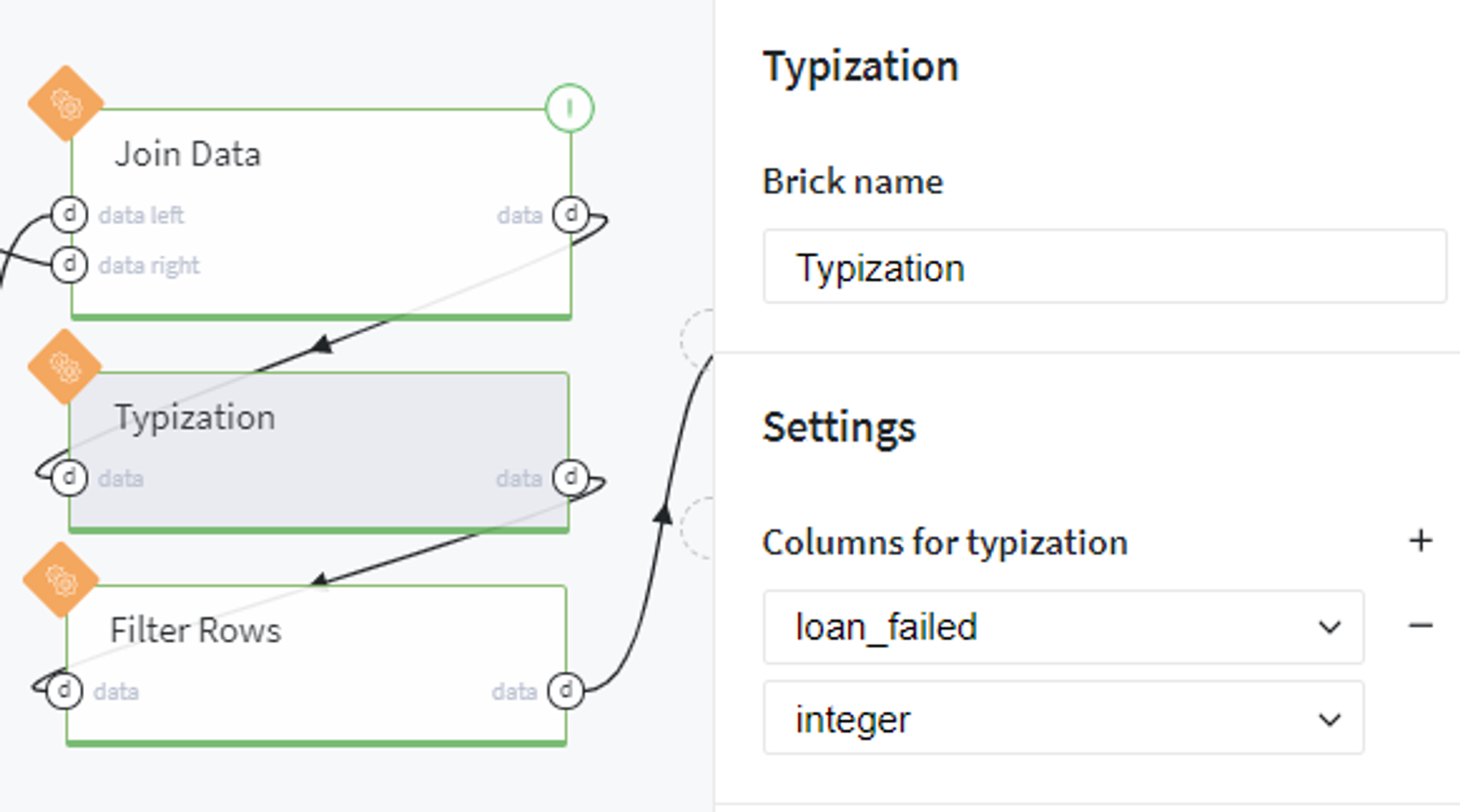
Convert the loan_failed column to integer data type:

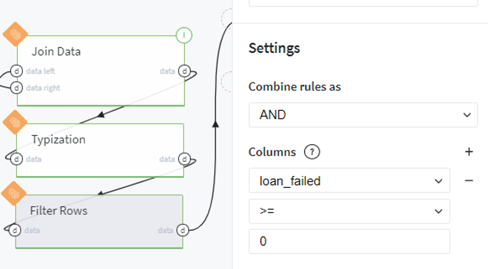
And, finally, exclude members with indicated uncertain loan status from our merged dataset:

Data Preprocessing

BRICKS:

Filter Columns

Missing Values Treatment

Pipeline

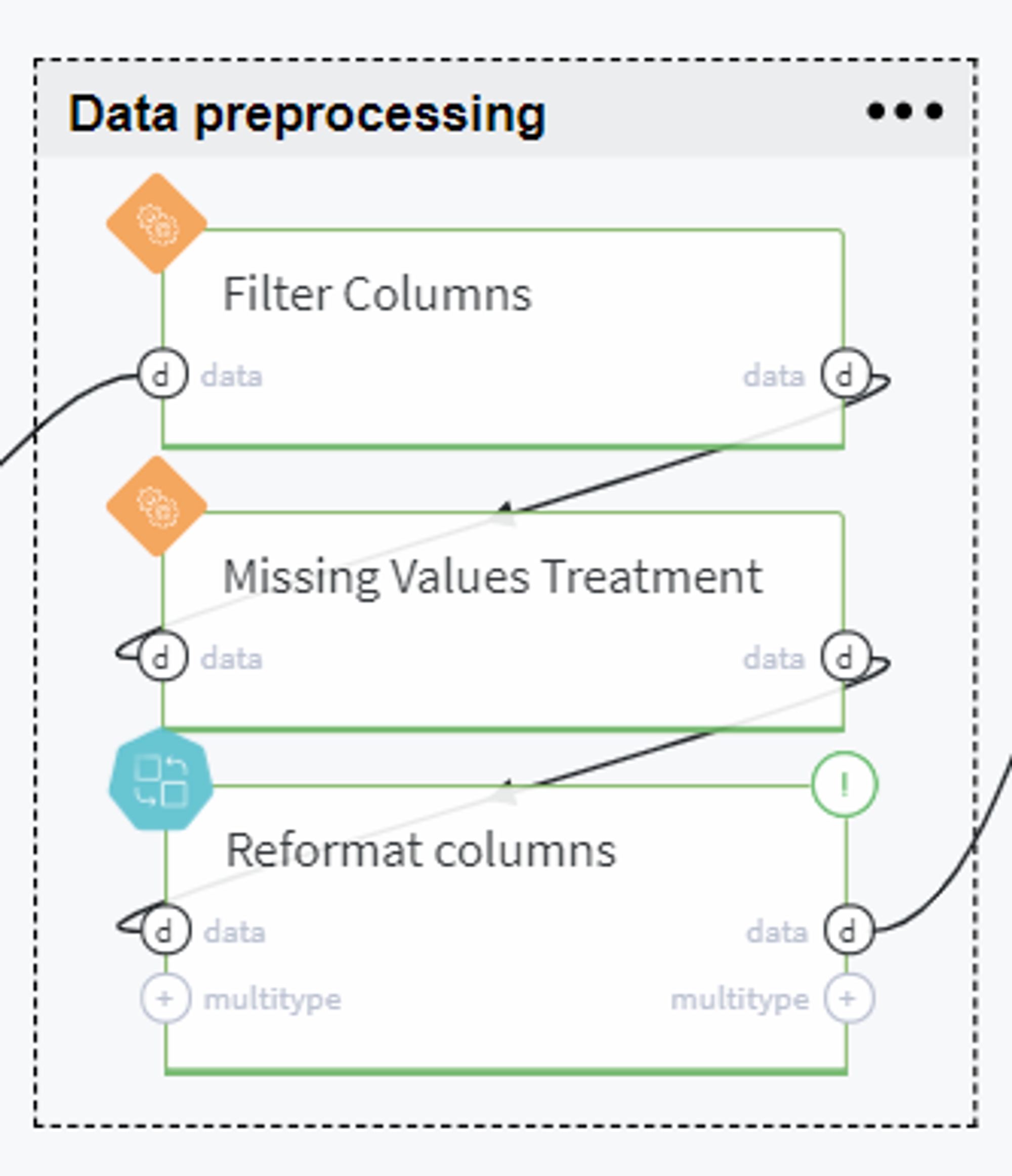
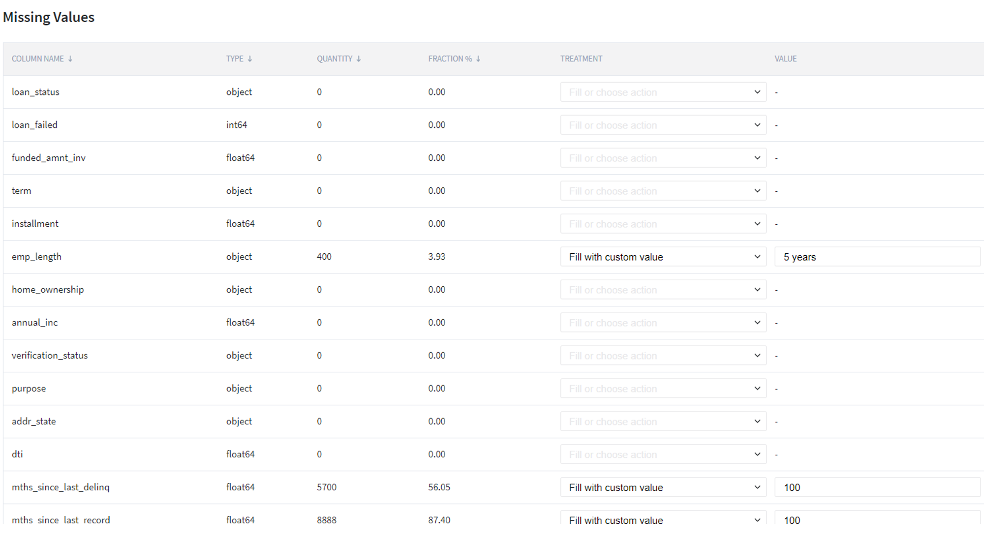
From the obtained dataset with the encoded target variable and explanatory features, we exclude the uninformative variables and handle missing values. In particular, for the latter, we propose to delete the columns which are fully empty in our table (e.g. the columns open_acc_6m, open_il_6m, mths_since_rcnt_il, total_bal_il, il_util...), fill with 0 (zero) the columns total_rev_hi_lim, tot_coll_amt, tot_cur_bal, fill with 100 the columns mths_since_last_delinq, mths_since_last_record, and fill the emp_length with value 5 years.

After that we reformat the columns which contain some useful numerical features, however, are presented in our dataset as text, and introduce a new variable Loan to Income rate (lit). All these steps are merged in one Pipeline brick named Reformat columns:

BRICKS:

Apply Function

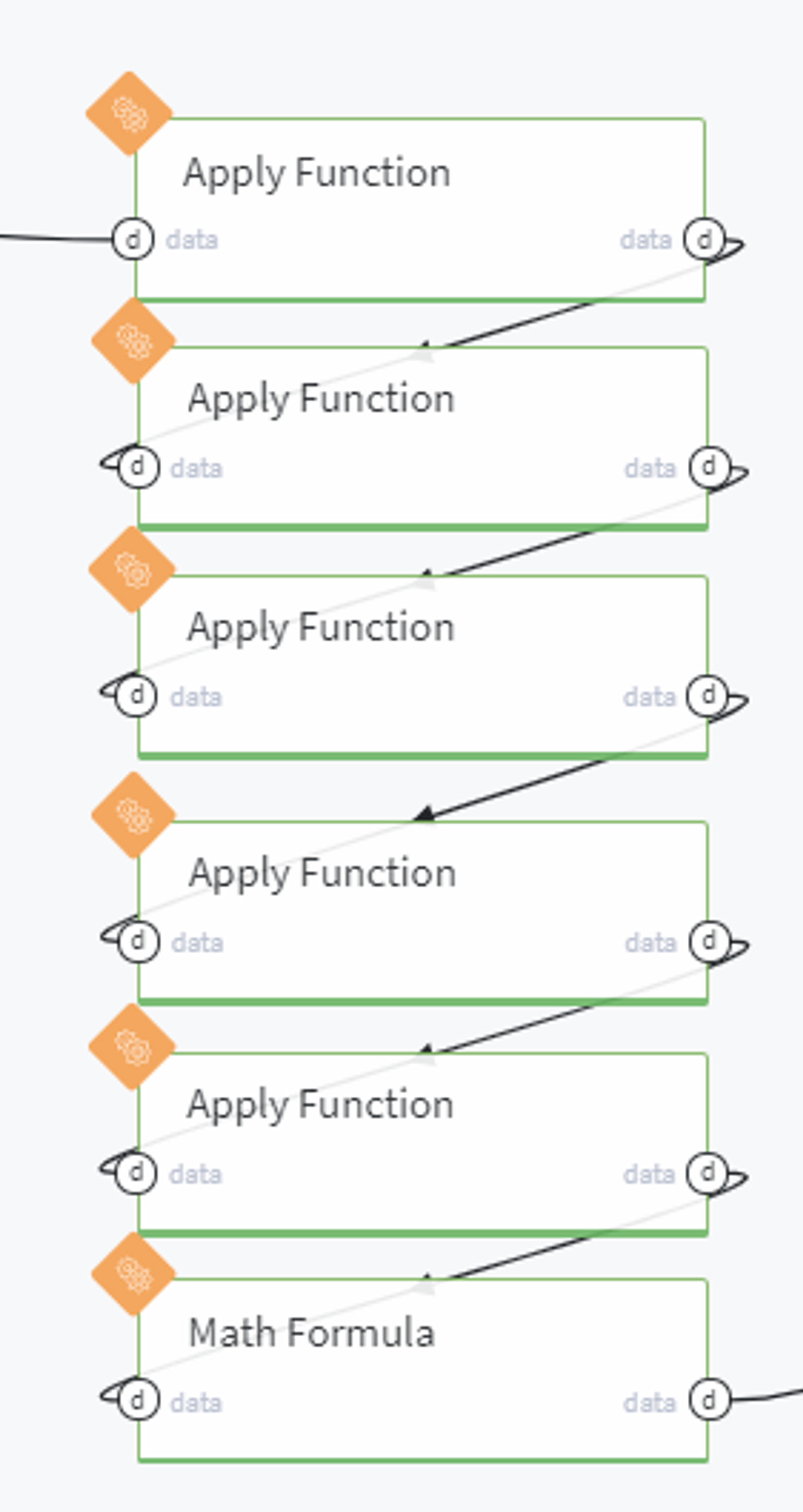
In this pipeline, we sequentially edit the textual columns by removing the parts of the text and leaving the numeric value, for example here we transform the column term:

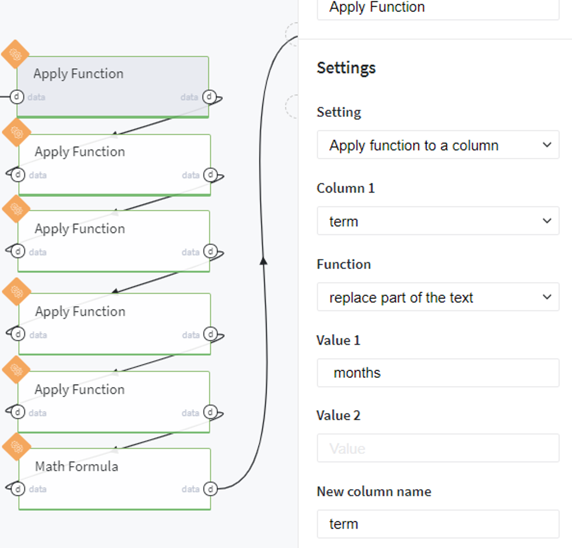
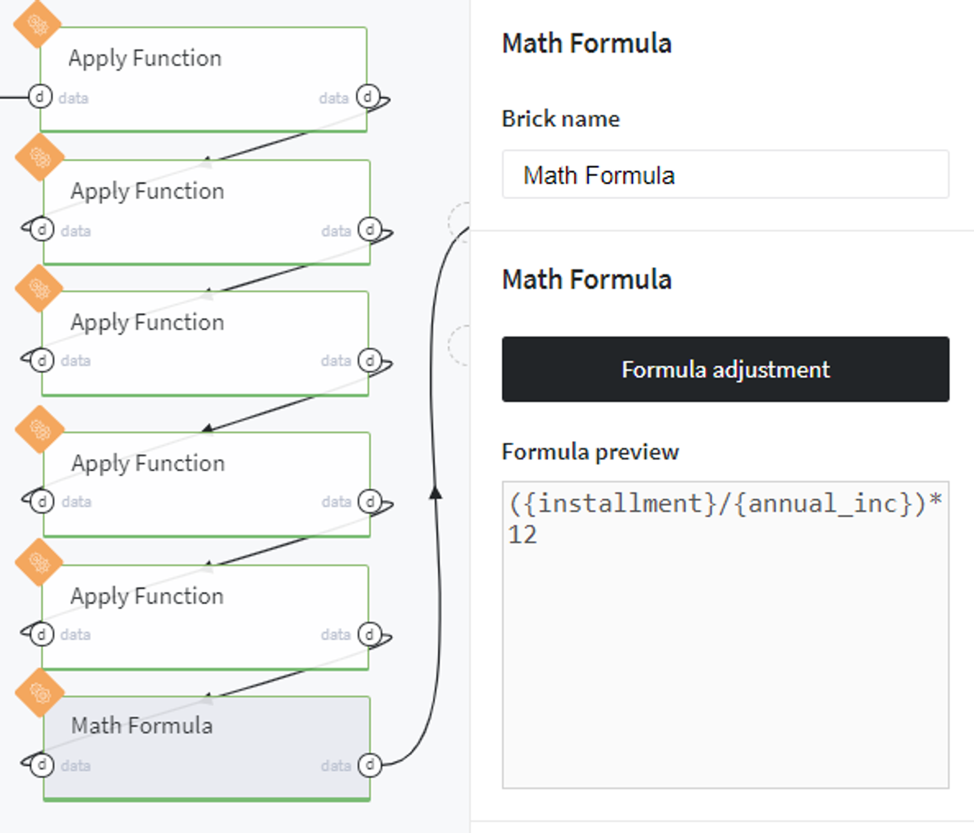
In the end, we create a new column lti using the following mathematical formula:

Feature analysis

BRICKS:

Typization

Pipeline

On this step we analyze the given variables and select the most informative ones to be used further for modeling.

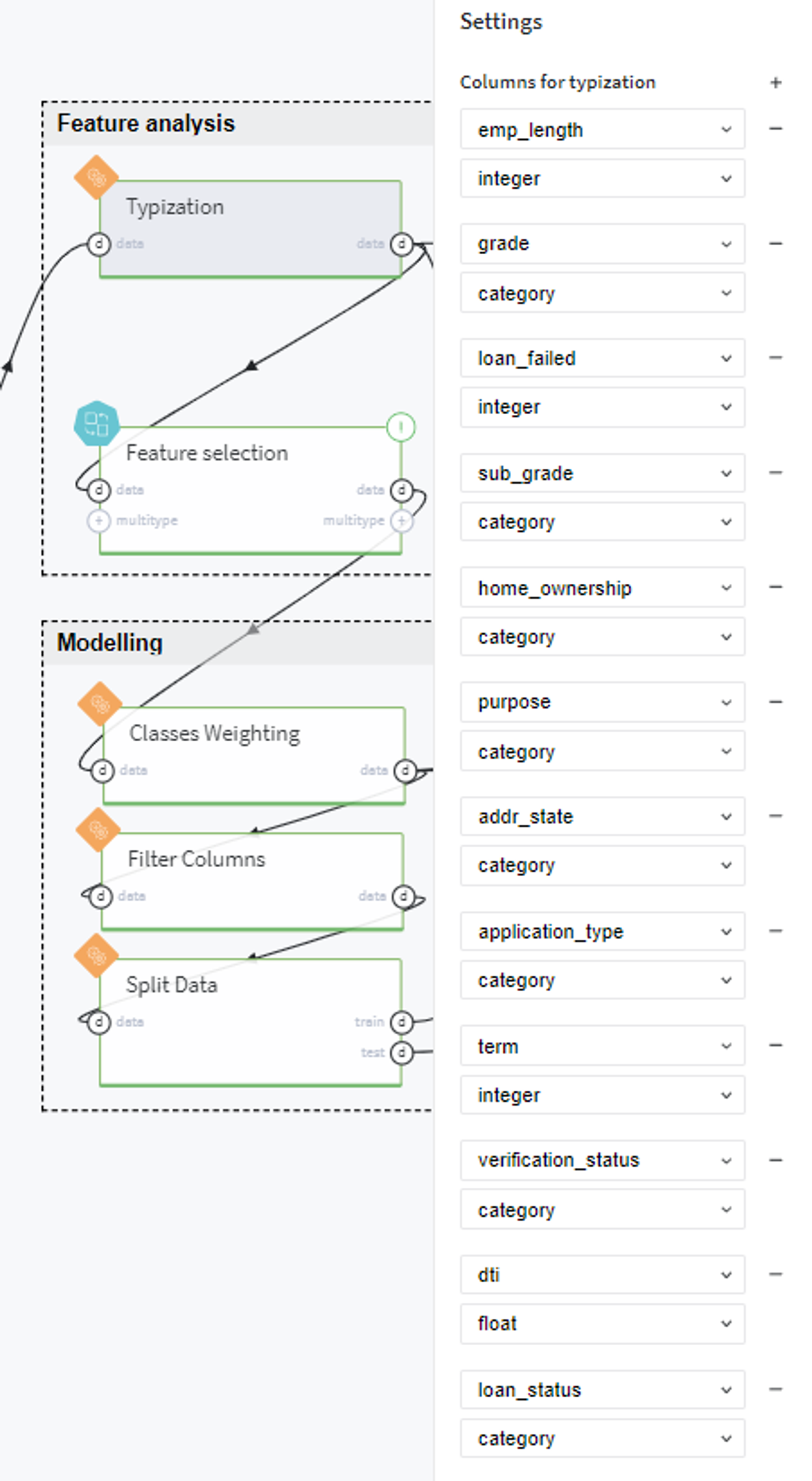
To start with, we transform the features to the appropriate types as follows:

Then we perform some visual analysis of our variables and their relationship with the target variable.

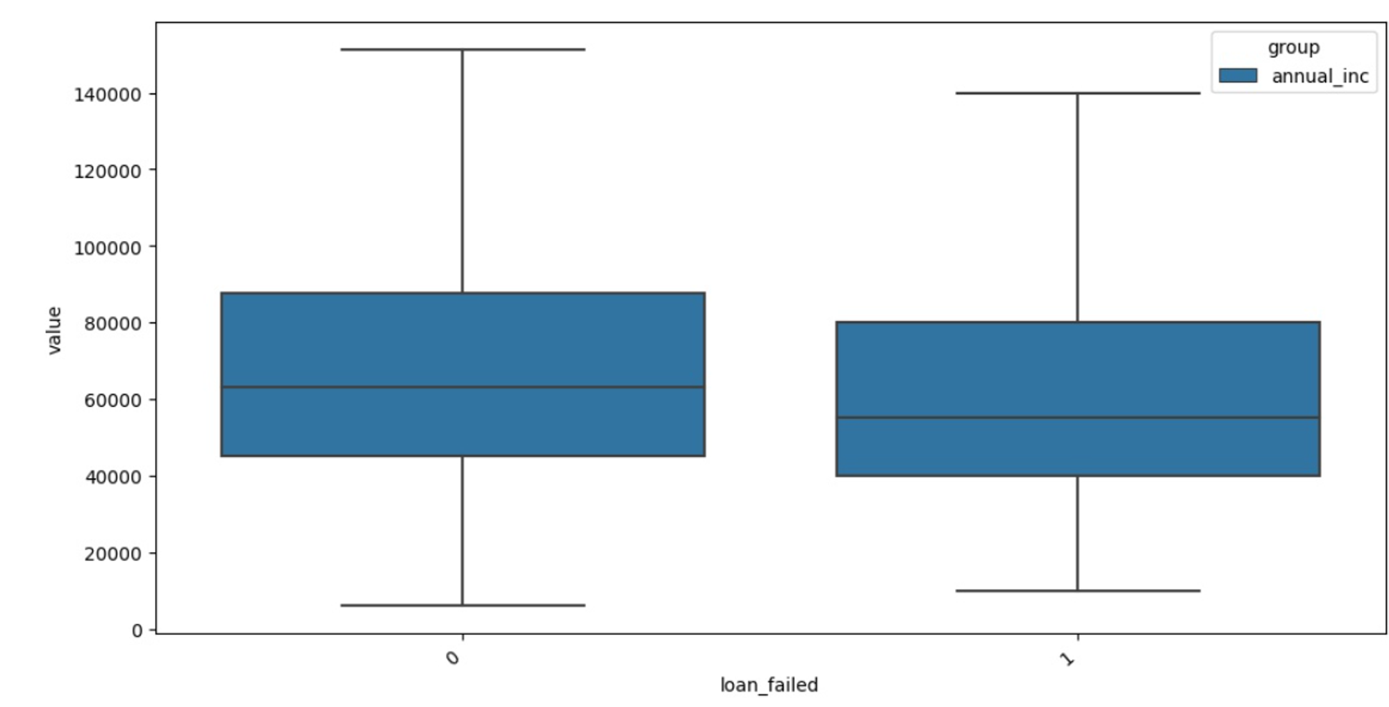
For example, this can be done using the heatmaps or box plots, for example, to see how the personal annual income affects the customer creditworthiness we use the chart with the following settings:

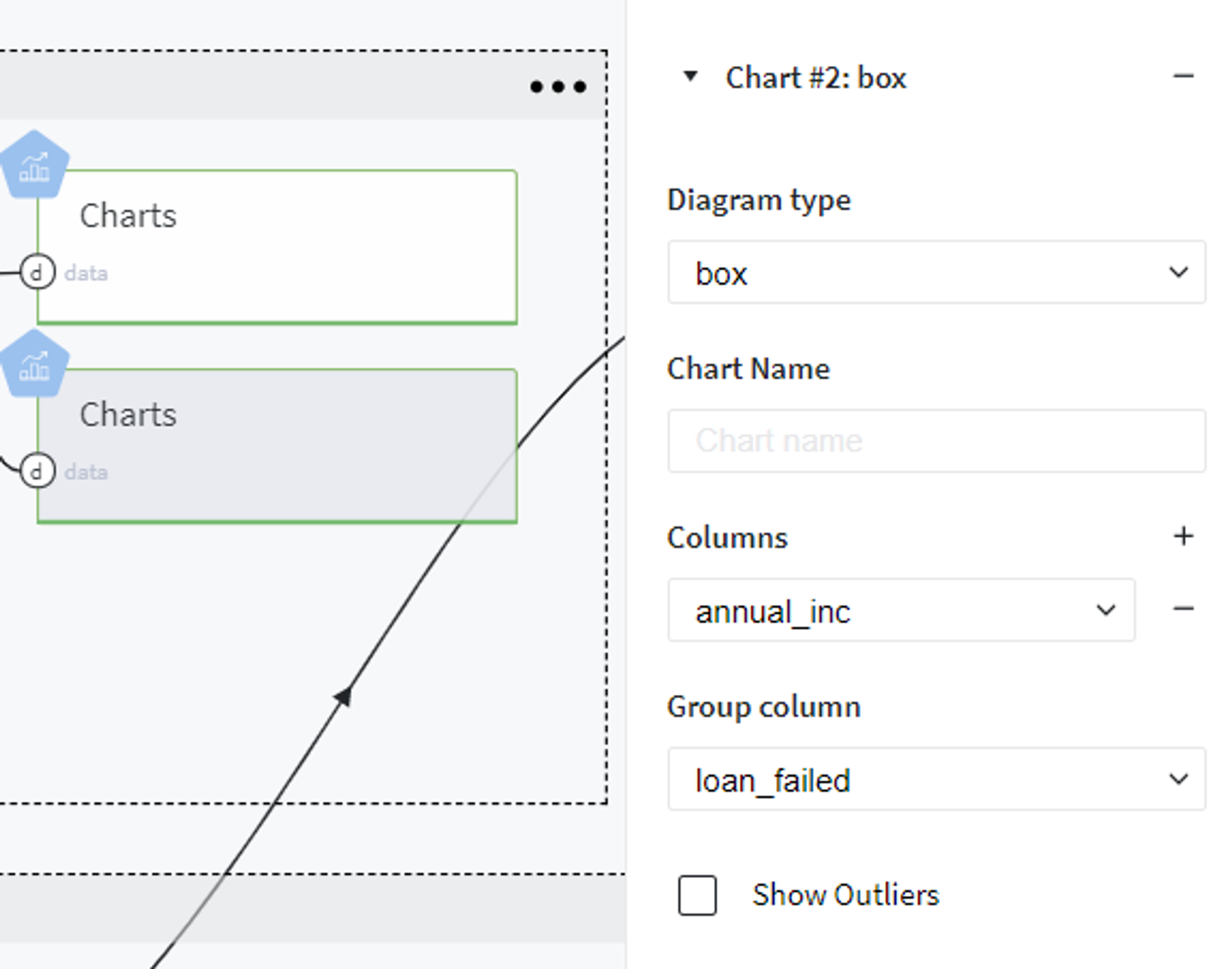
And receive the following plot:

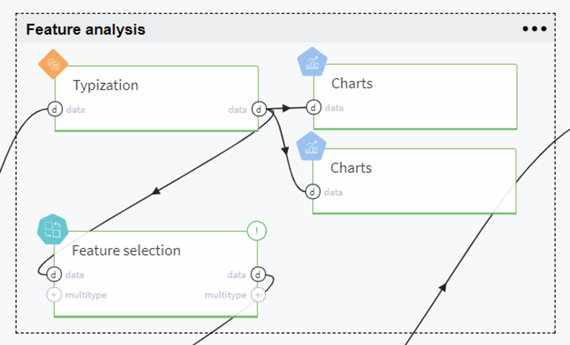
Now we are ready to select the features for modeling. This step is performed with Pipeline brick named Feature selection, that is expanded in the set of bricks as follows:

BRICKS:

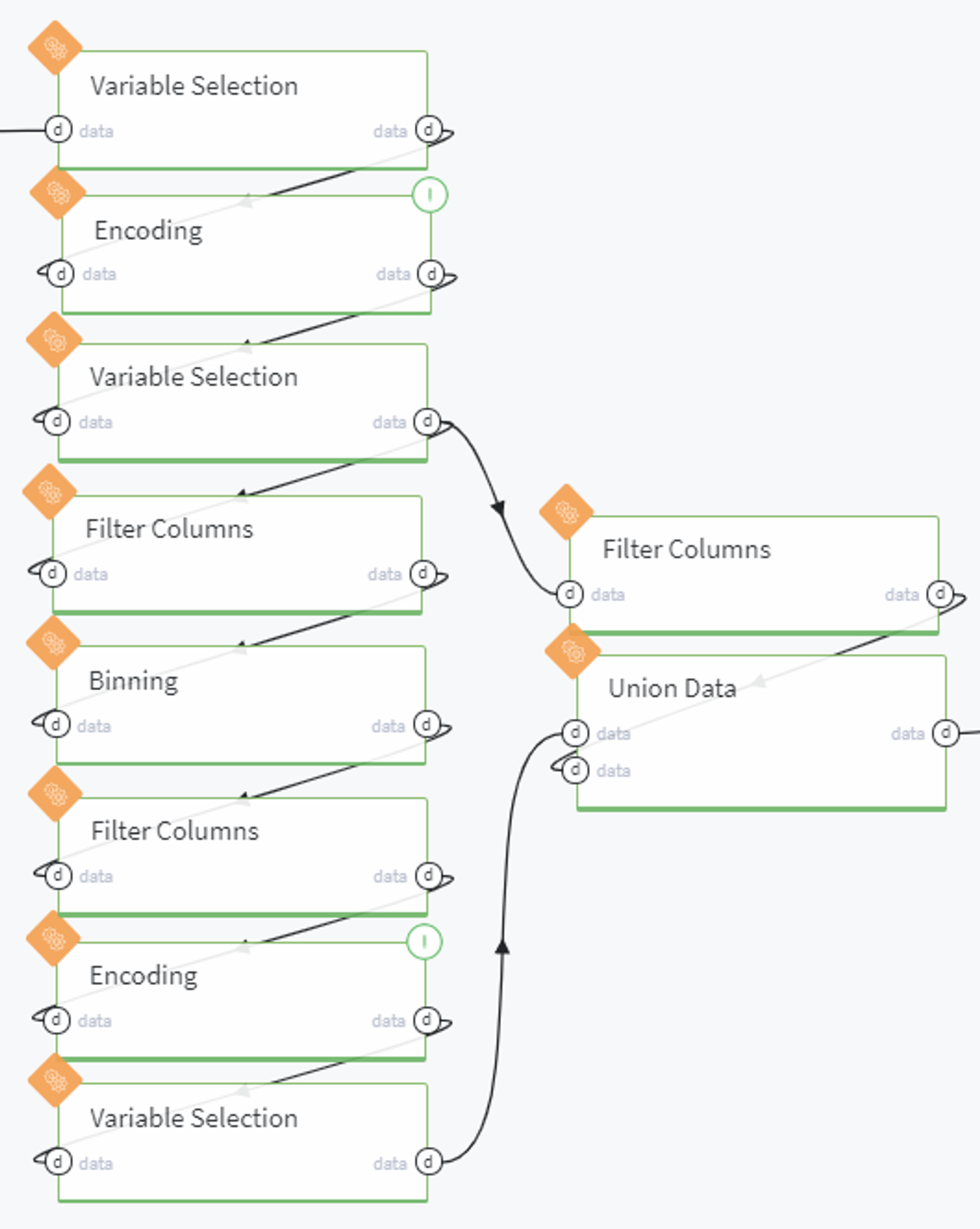
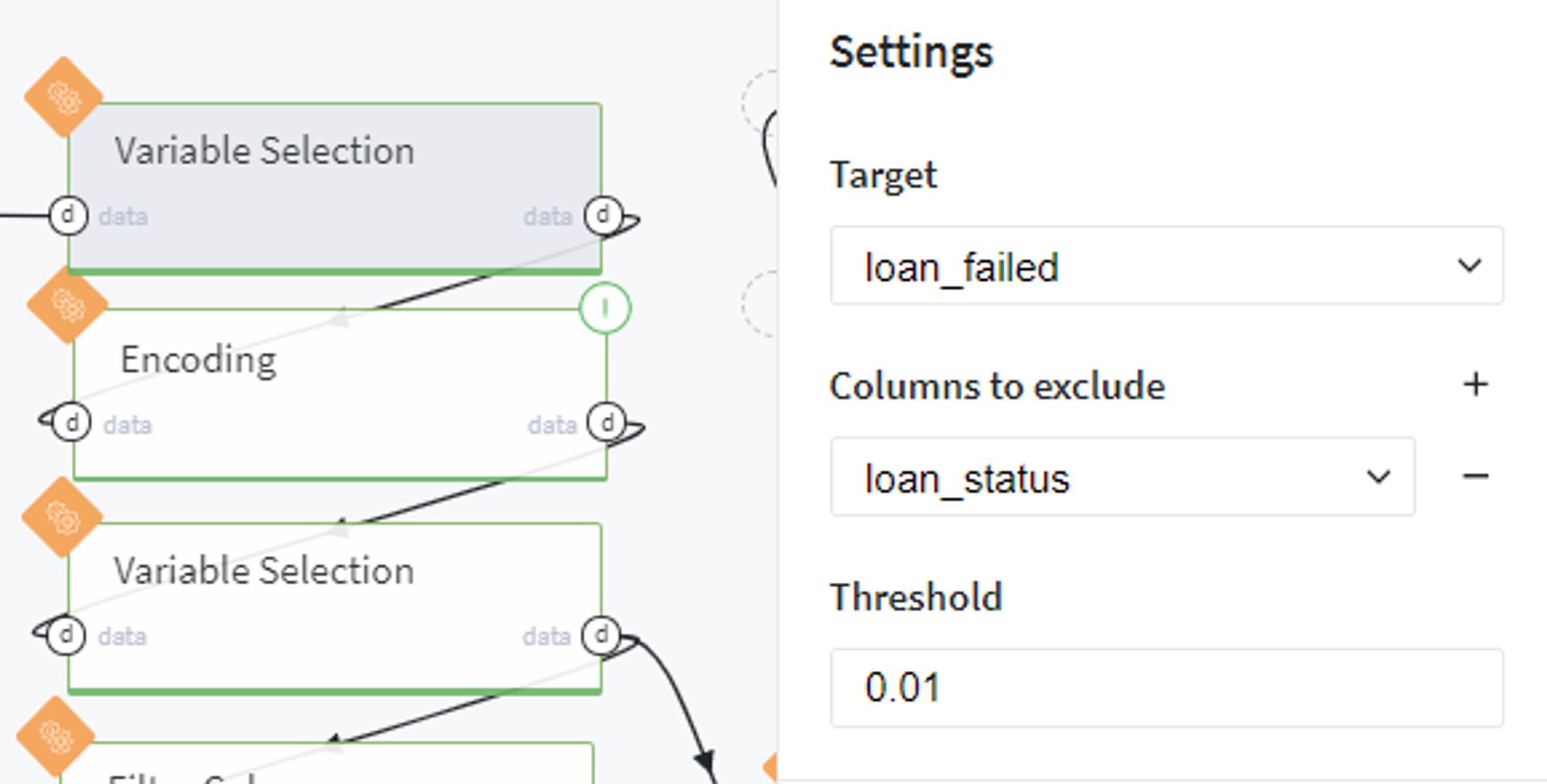
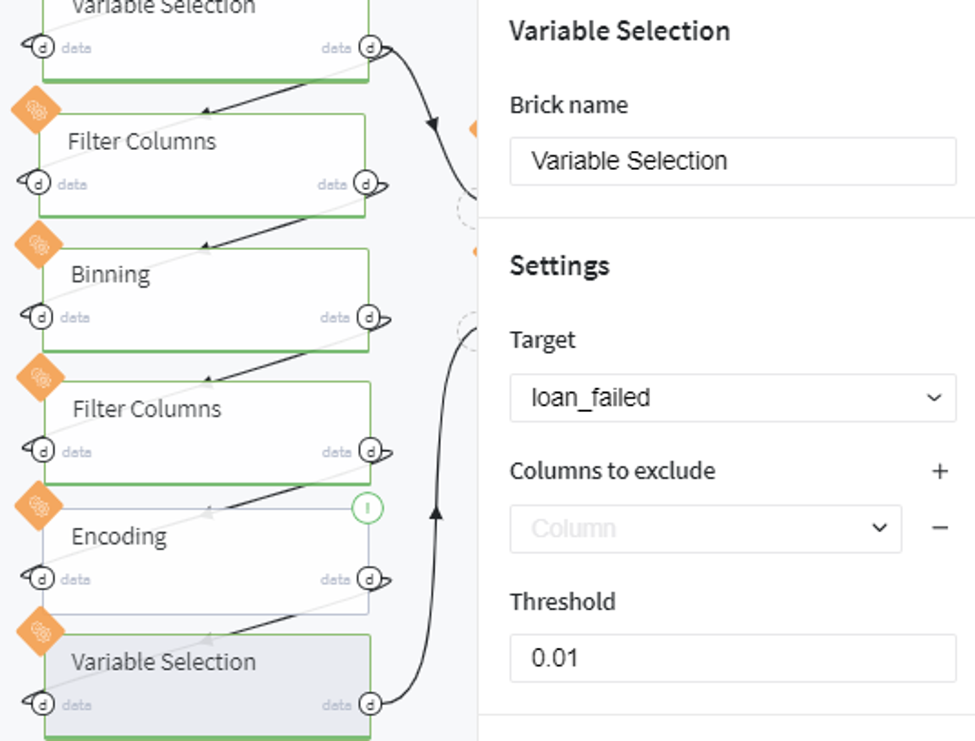
Firstly, we select the informative features among all possible variables by the information value (IV) criteria with threshold equal to 0.01:

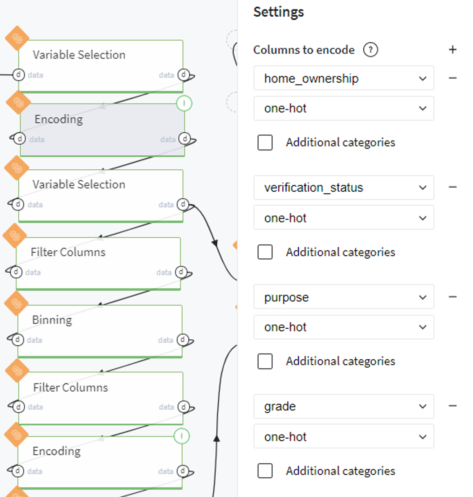
Encode the categorical features with one-hot encoder:

Then we repeat the procedure of feature selection but with newly created category columns:

After that we split our table and select the numerical features into the separate dataset to apply the quantile-based binning with respect to the target variable (loan_failed) further:

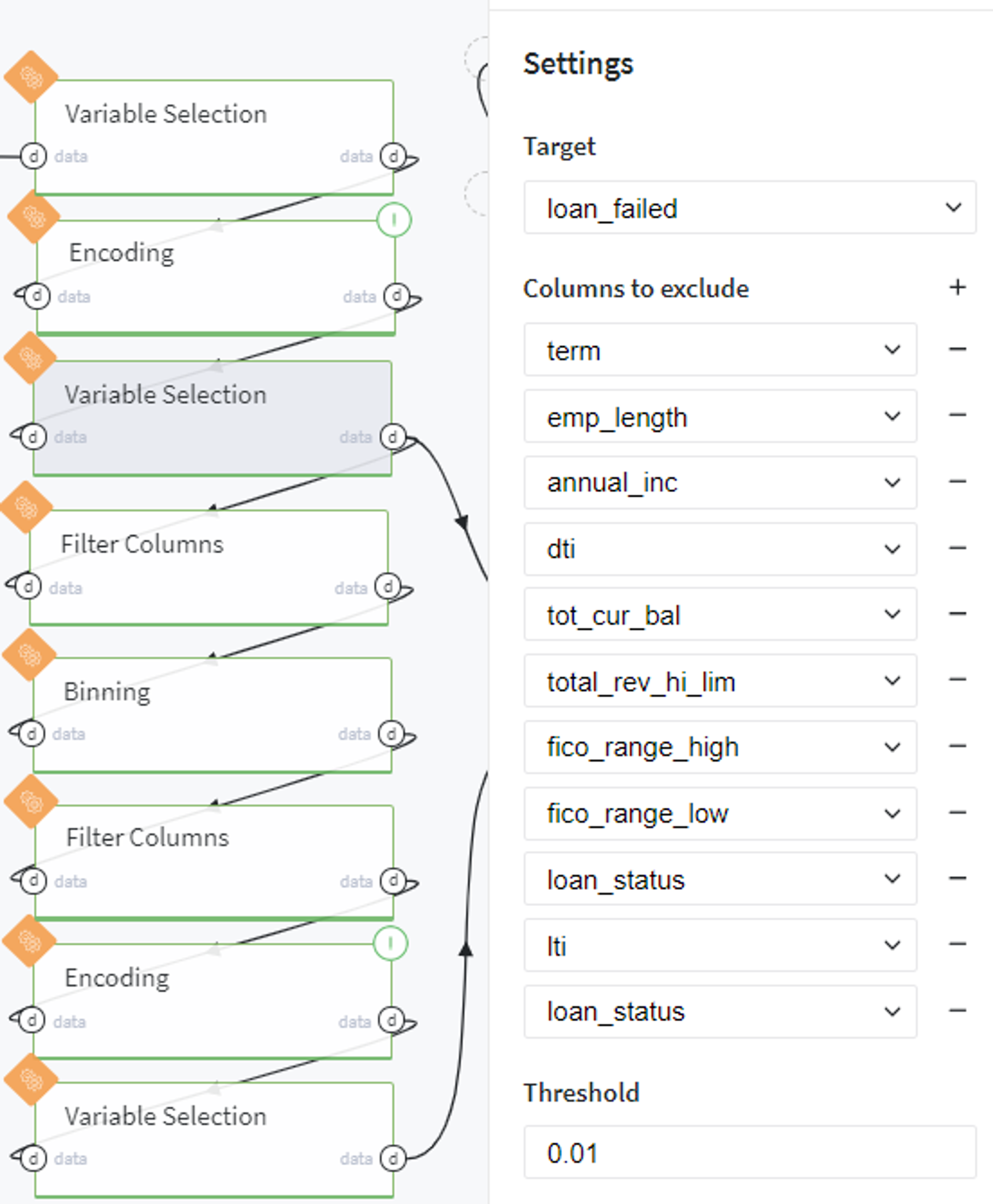
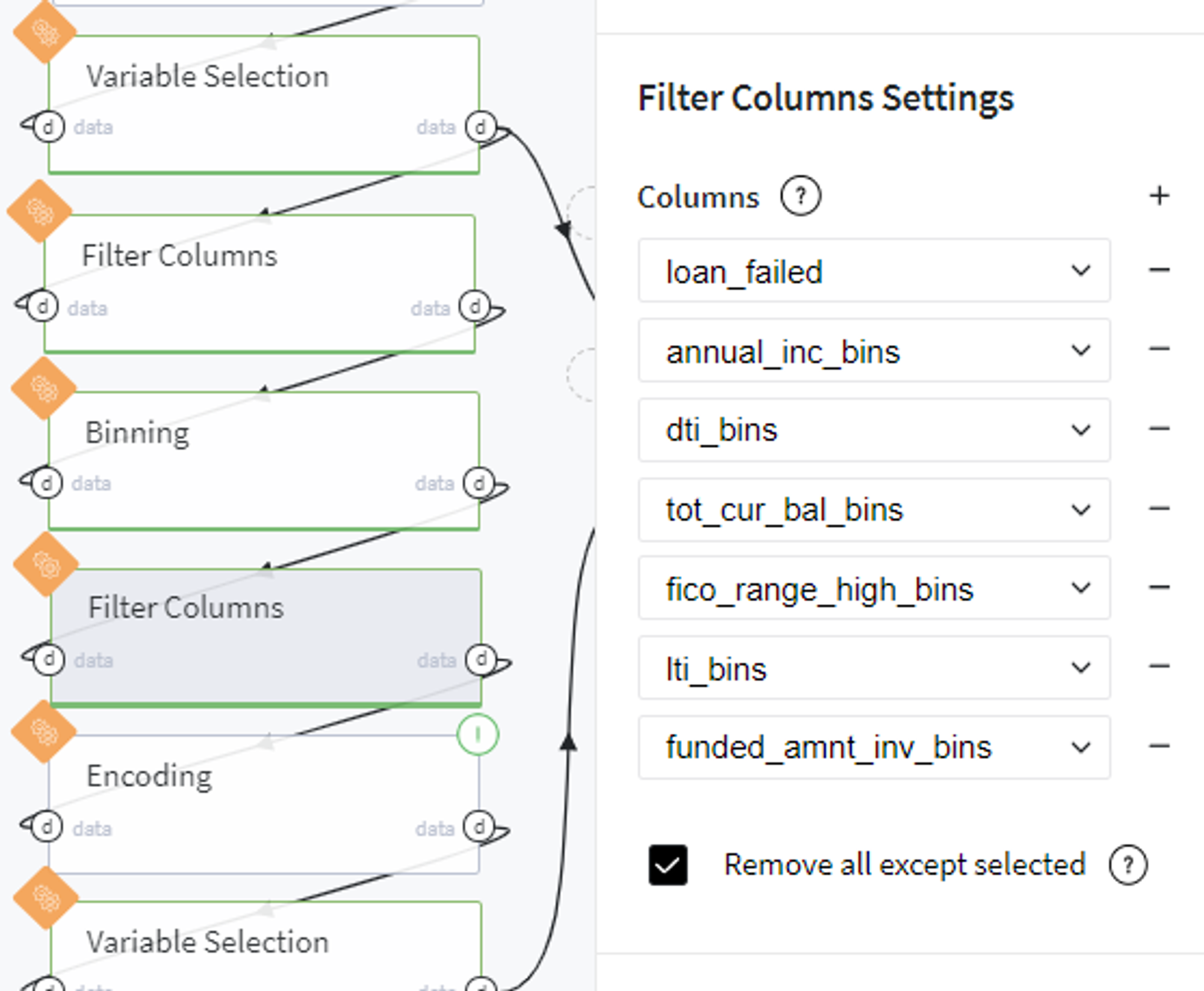
At the same time, we filter out the selected columns from the initial dataset into another separate table:

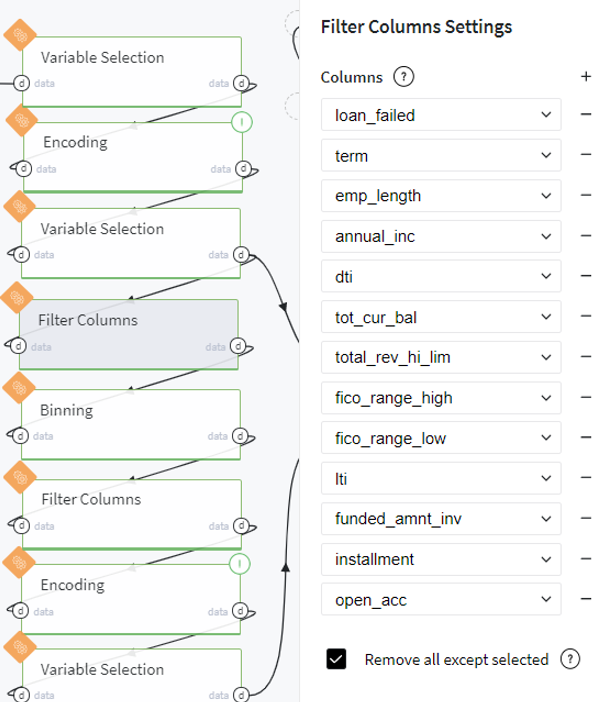
After performing binning, we filter out the produced bins columns:

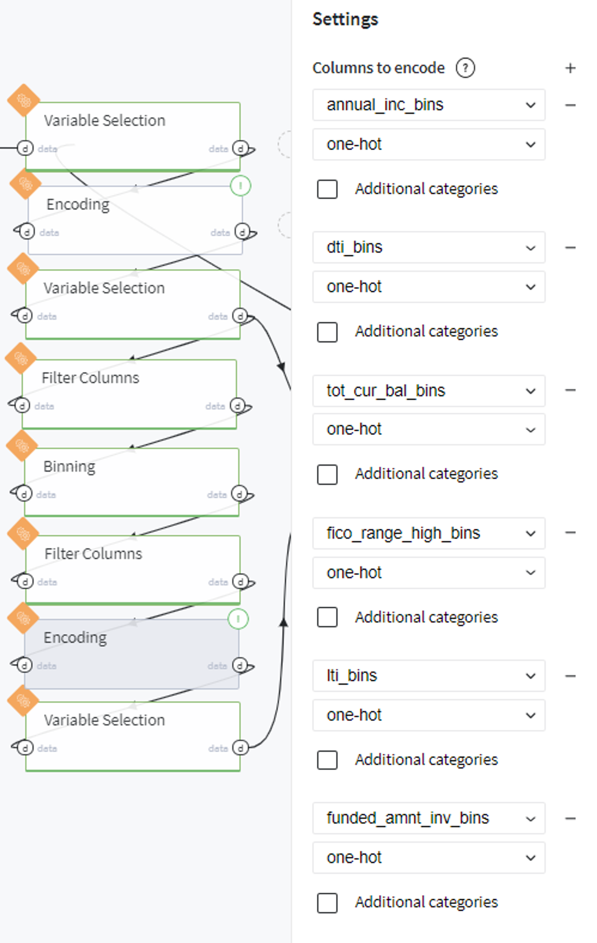
And transform them to dummy variables with one-hot encoder:

Similarly, we apply variable selection on the obtained bins categories:

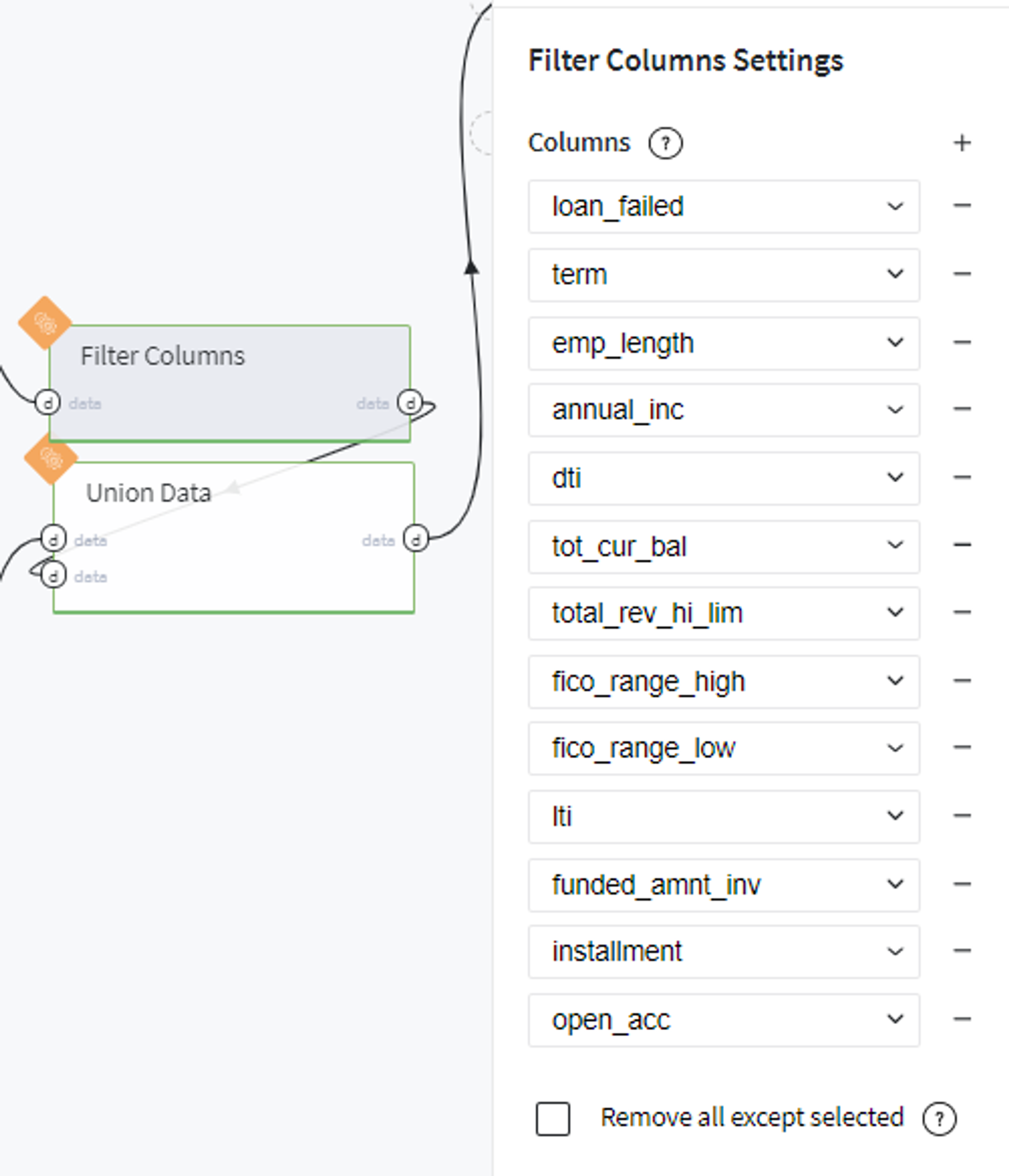
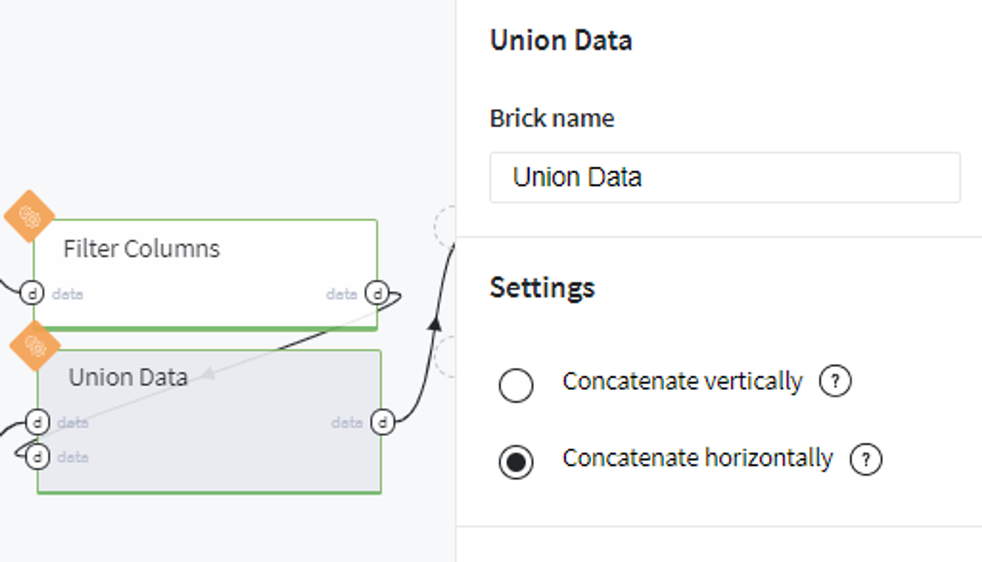
And merge the most informative bins with hold-out previously table as follows:

Thus we obtain the full dataset with the target variable and most informative encoded explanatory features.

Modeling

BRICKS:

Filter Columns

Split Data

Predict

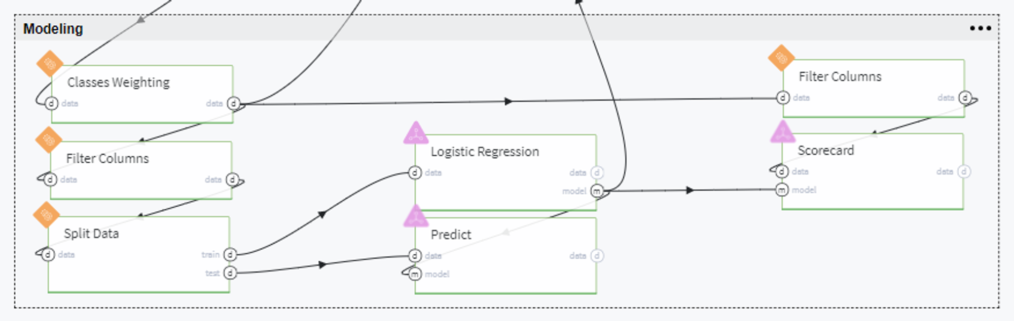
On this step we have a full dataset that we will fit into the model, but, previously, we need to tackle several issues.

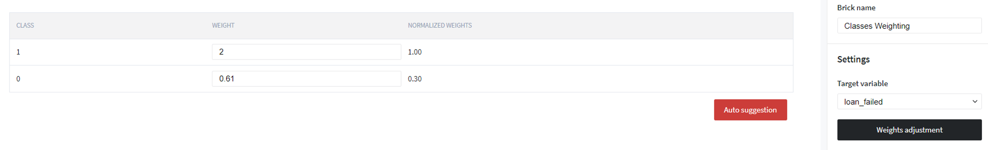
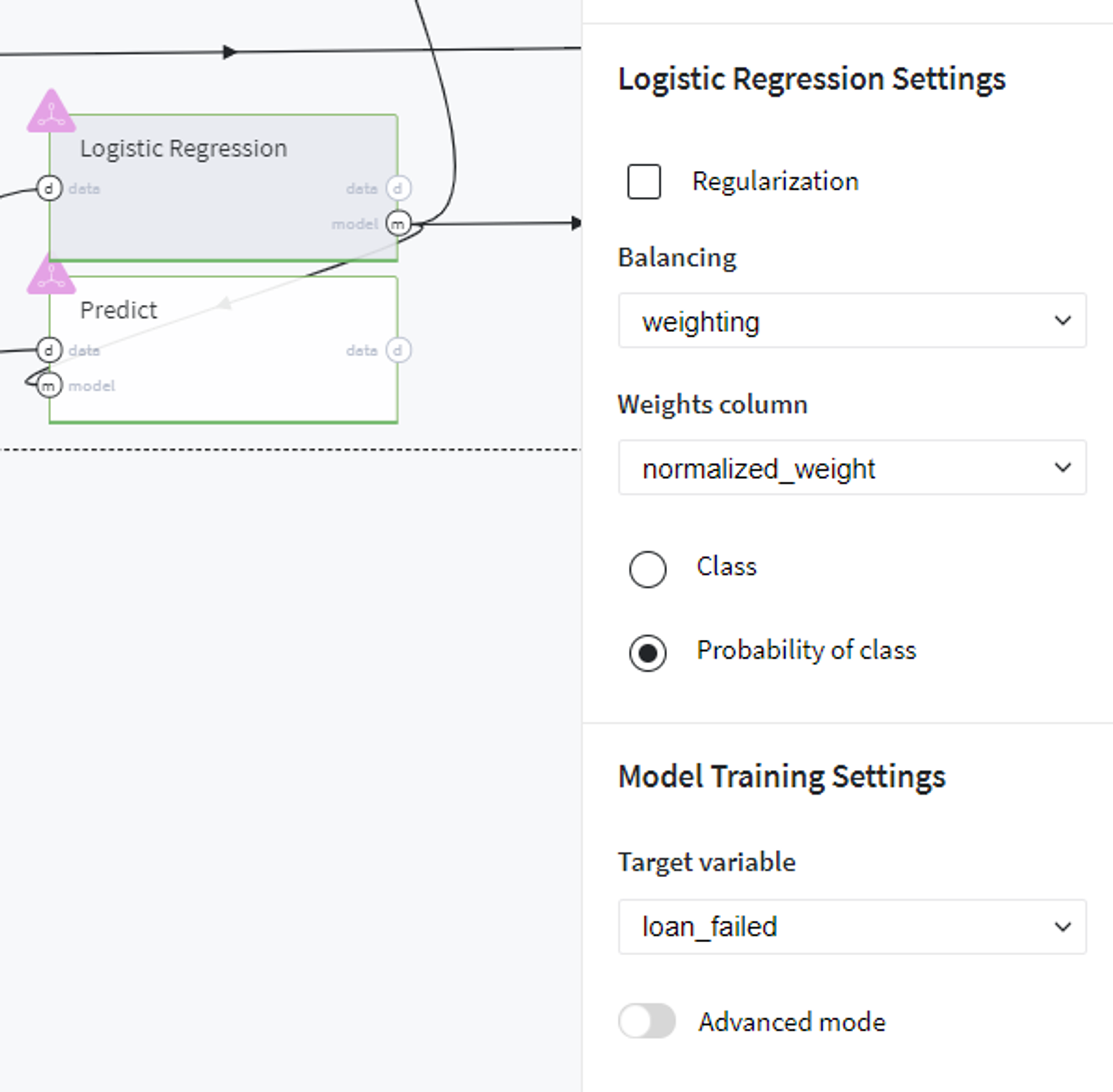
First of all, since we are dealing with imbalanced classes (the number of people who failed the credit repayment is considerably less than those who fully covered the loan), we assign the following weights to the classes we need to predict:

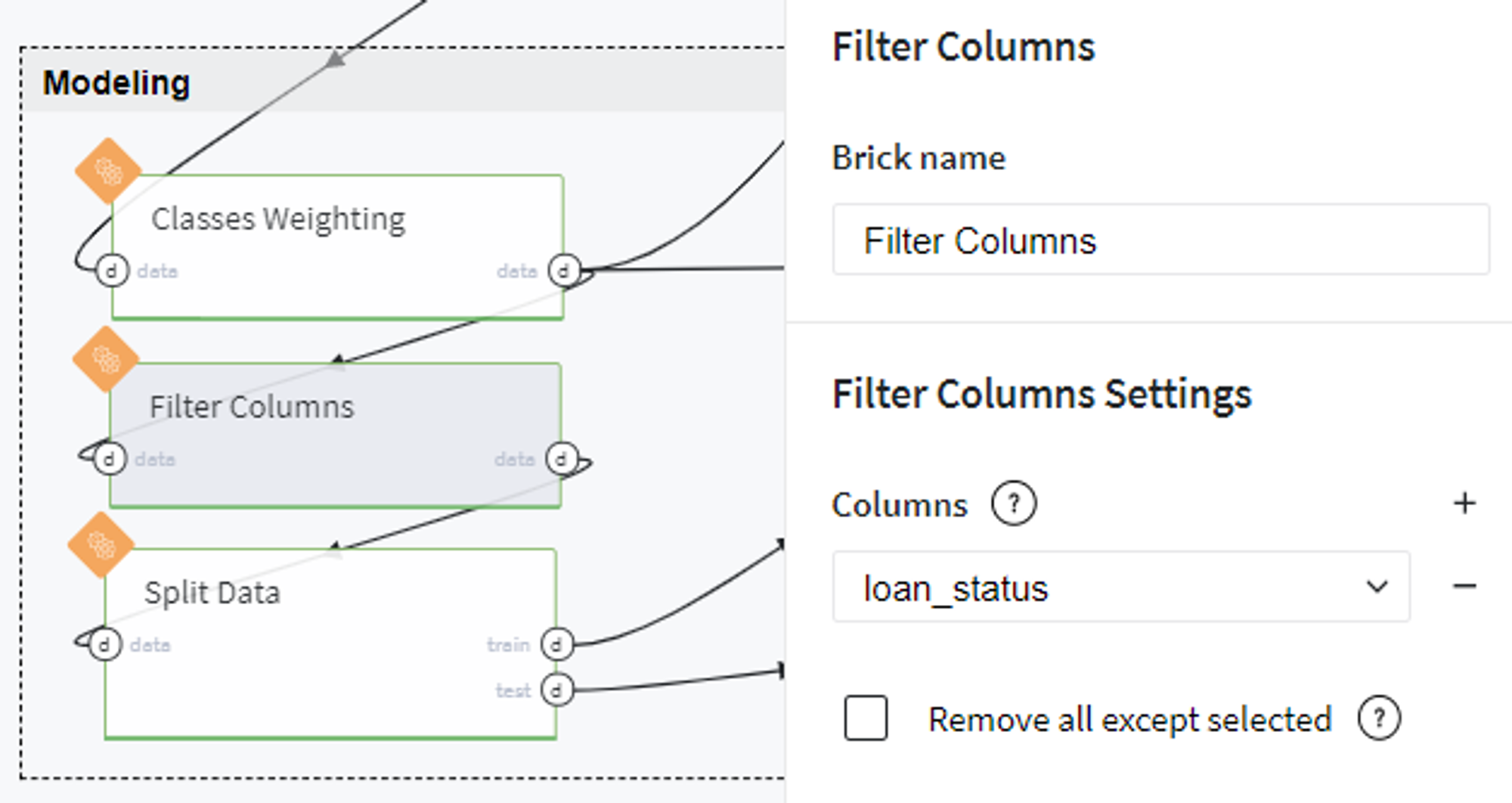
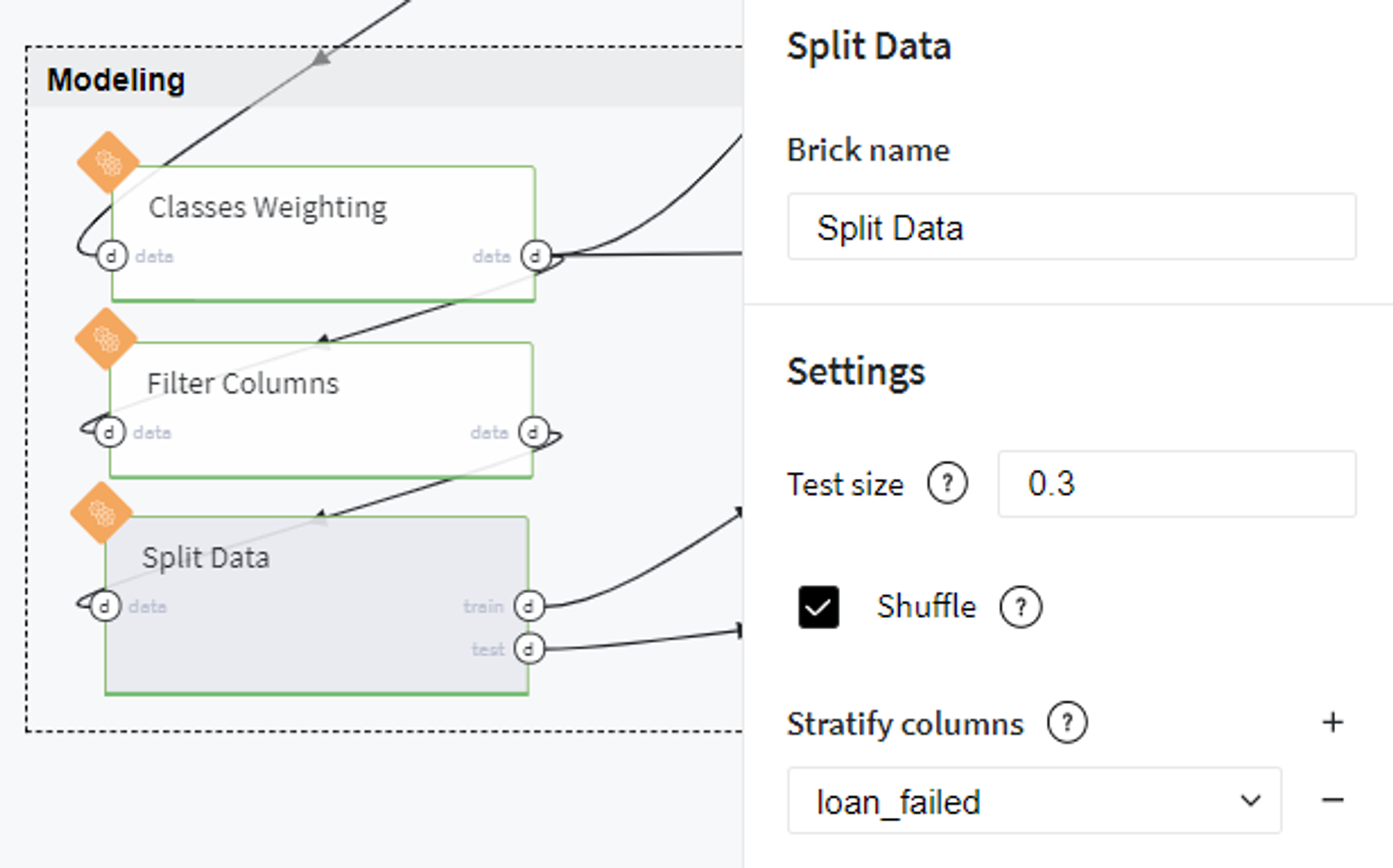
Then we exclude the textual column loan_status from our dataset and split the data into train and test sets with stratification by target variable:

Next, we fit the train set into Logistic Regression model with defined classes weights and target variable.

After running the pipeline we can review the performance of the built model on the train data using Model Info → Open view button on the Logistic Regression brick tab.

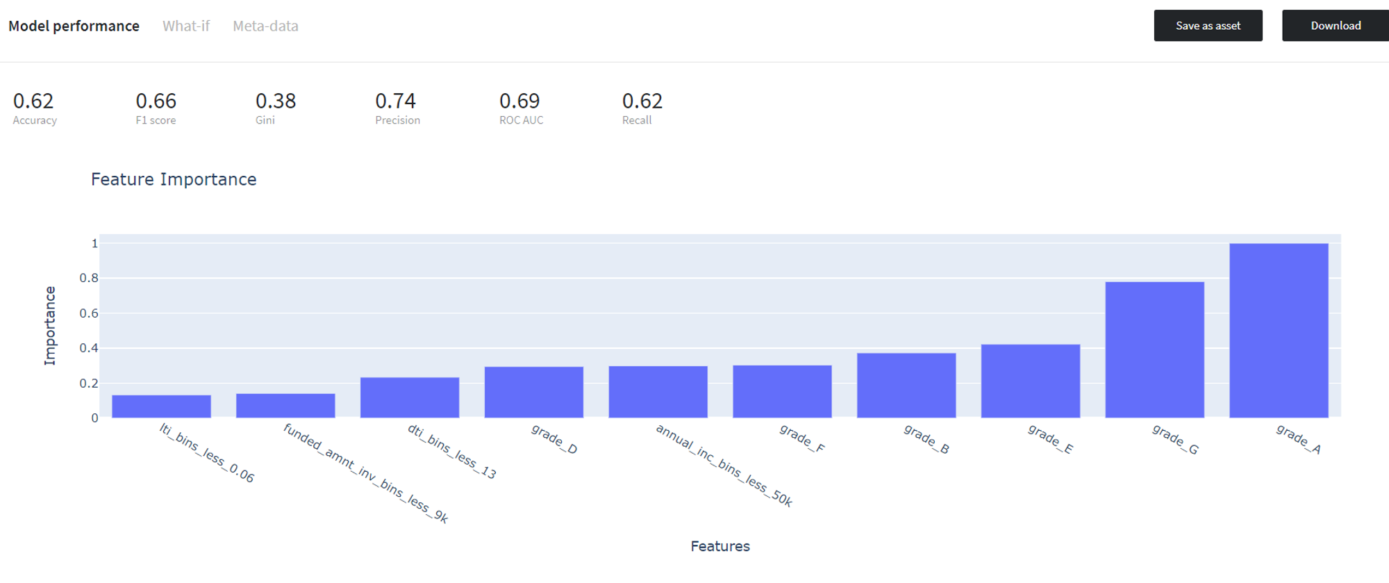
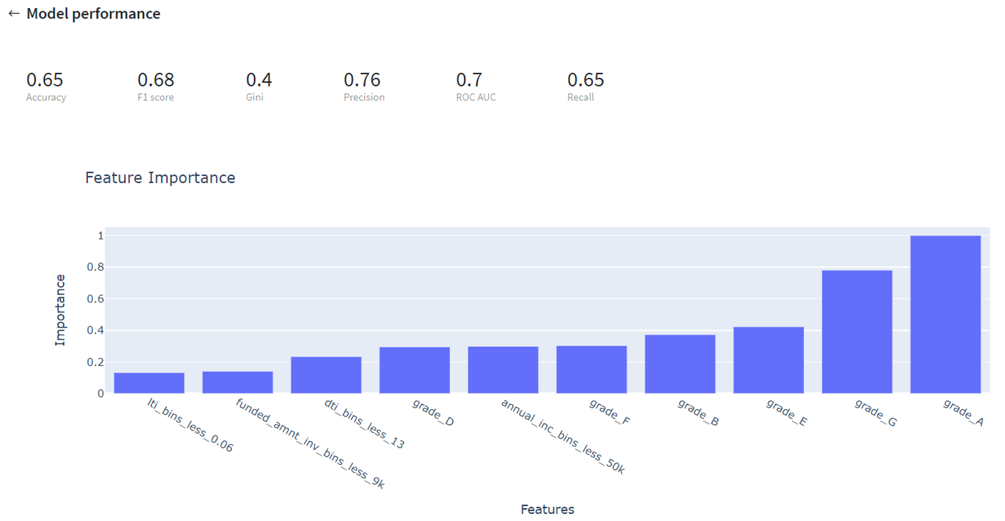
Then we validate the trained model on the test data and assess its performance via Predict Stats → Model Performance tab on the Predict brick:

Despite looking at prediction metrics, we also can transform our model into the Scorecard, which provides a clear understanding of the contribution of the different factors to the final Credit Score of the customer.

For doing so, we prepare a dataset with features for which we evaluate the contribution with respect to the target variable and transform the coefficients of the trained Logistic Regression model to the factors' scores via Odds Scaling:

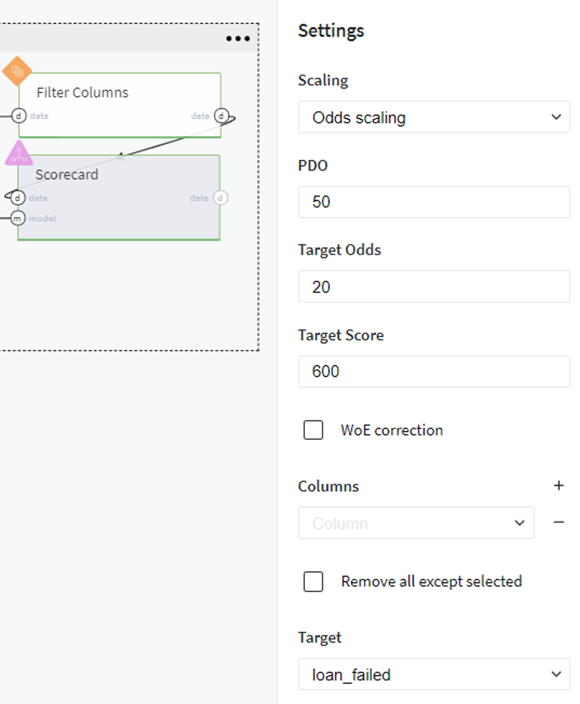
The final Scorecard looks like:

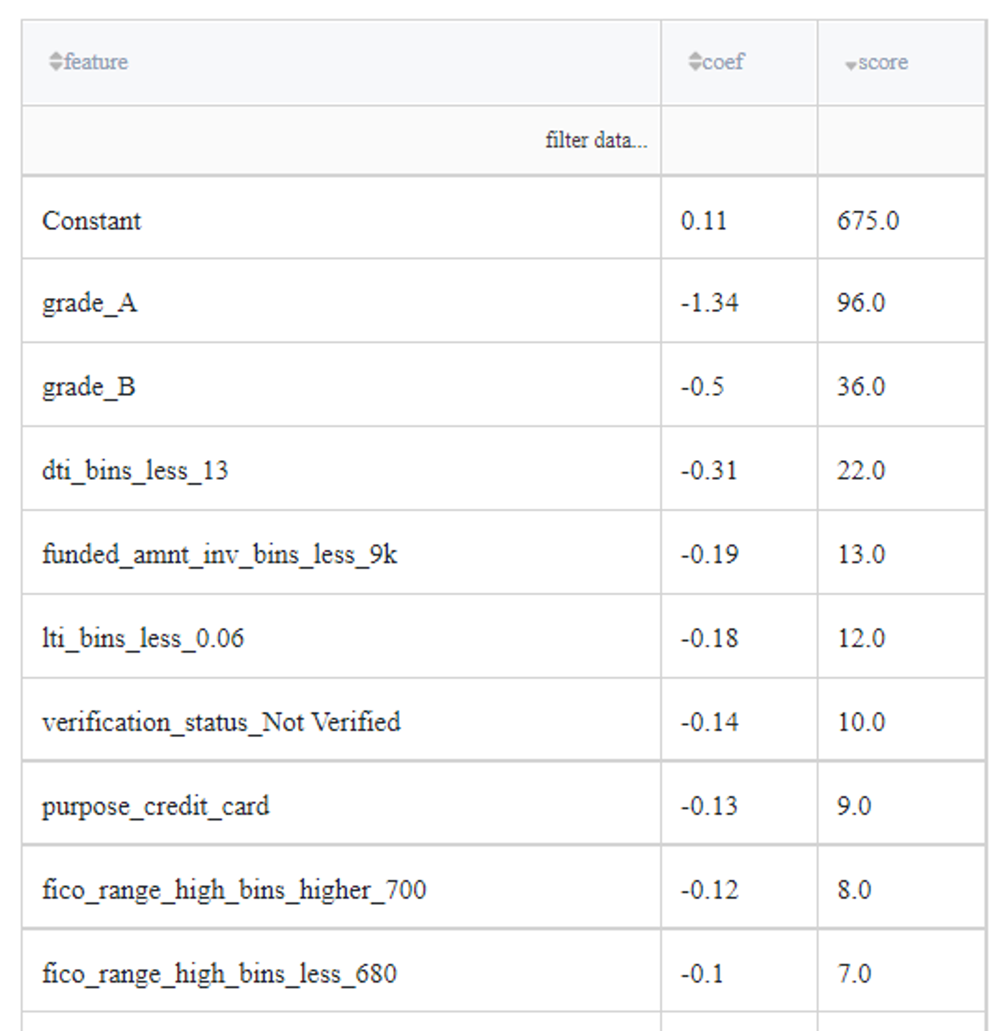
Note, that scores are opposite to the regression coefficients, because of the opposite purpose of the assessment - the LogReg model asses the Credit Default Risk, but the ScoreCard - the creditworthy.

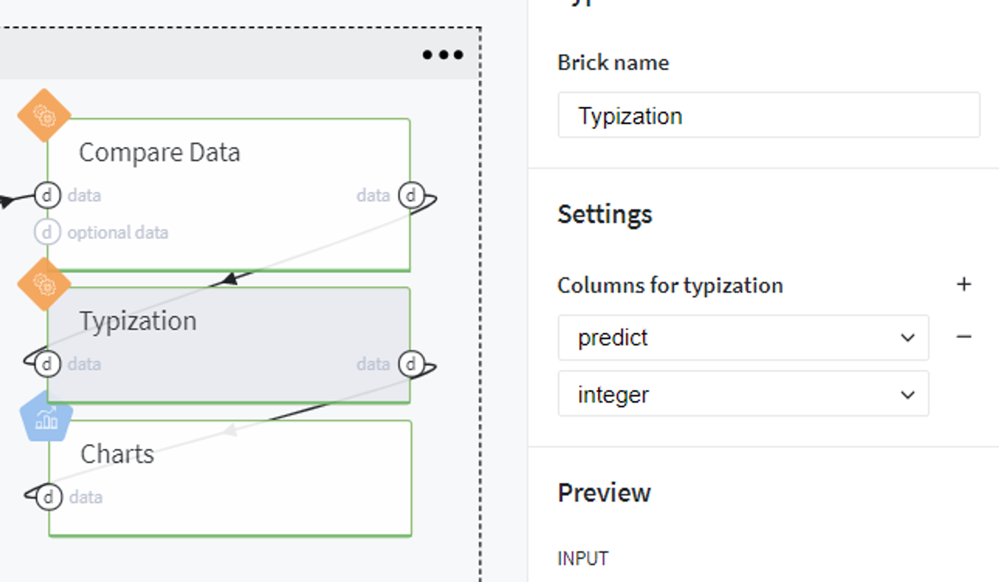
Results visualization

BRICKS:

Predict

Compare Data

Typization

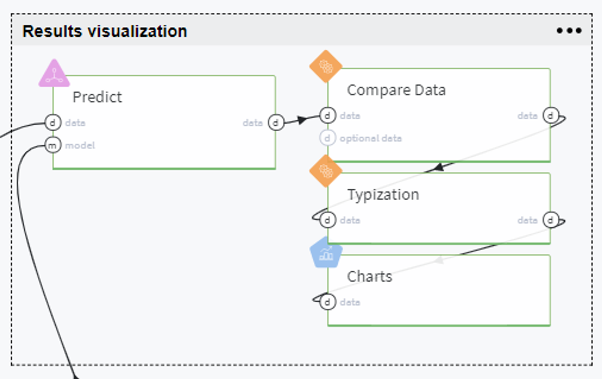
In order to visualize the results of our modeling and analyze the dependencies between predictors and target variable, we generate several plots using the output of the Predict brick with predictions on the full dataset (obtained before its split to train/test sets).

Since the trained logistic regression model returns the probability of class as the prediction, we firstly transform our predicted values into the binary category. Here we use the standard threshold (0.5), so consider the customer to be creditworthy if his\her predicted probability to fail the loan is less than 50%:

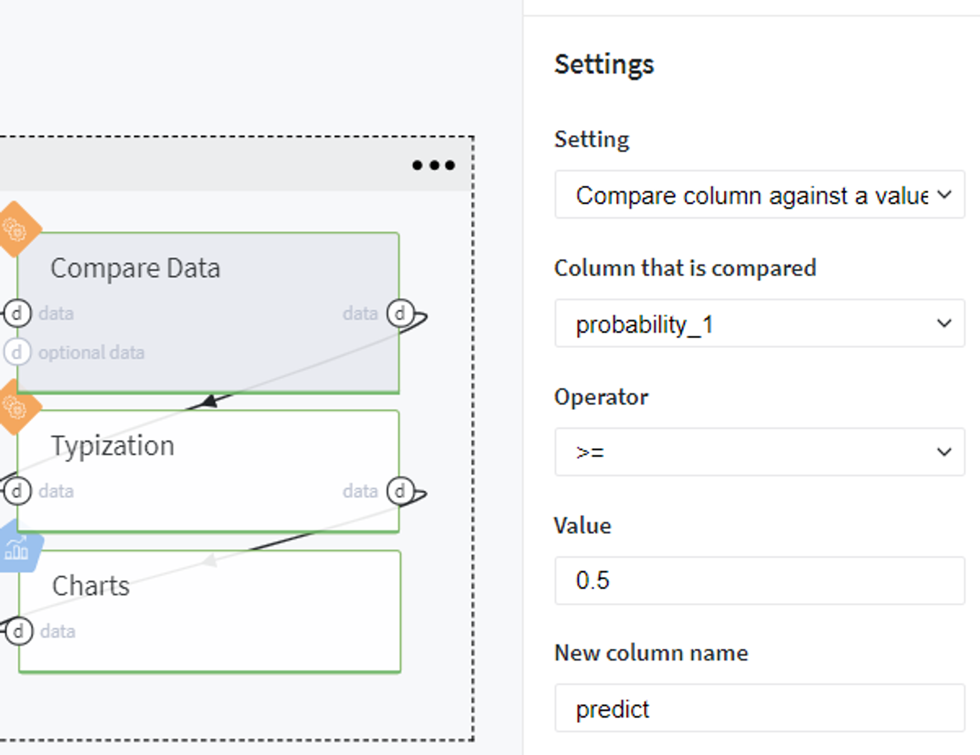
Then we transform the type of the newly generated column predict to integer and build the plots using the Chart brick:

Model Save and Deployment